Adaptable Curricular Exercises (ACE) for Quantum Information Science (QIS)
Research-based QIS instructional resources to support faculty, including those new to these topics, aiming to incorporate more active learning elements in their classes.
We have materials for two different audiences, depending on the type of course you teach:
QM Course: Are you teaching quantum mechanics in a physics department to (mostly) majors, and want to add a short unit on quantum information (e.g. quantum computing or cryptography) within your course?
QIS Course: Are you teaching a quantum computing/QIS course to students from a variety of majors (e.g. computer science, physics, engineering, math, etc.), and want materials for foundational topics?
And: if you teach undergraduate quantum mechanics to physics students and are looking for a suite of student-centered materials to help you with the entire QM course, please visit our Adaptable curricular materials for Quantum Mechanics site.
Standalone modules for introducing QIS in a QM course
Who is this for? An instructor teaching Quantum Mechanics who would like to add some quantum information science topics to their physics course. These materials are suitable for faculty new to these topics.
Topics:
 Qubits, Quantum Gates, and Teleportation(1 week module)
 Entanglement and EPR(1 week module)
 Quantum Cryptography(1 day module)
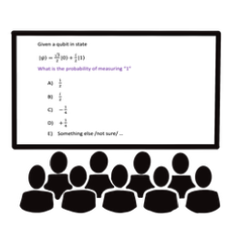
What materials are included in each module? Tutorials (online and paper versions), homework questions, exam questions, clicker questions (concept tests), and lecture notes for faculty.
When should I use each module in my class? Each is standalone - materials can be taught without any prerequisite material from the other modules. You can find examples of how other instructors have used these modules in the FAQ for each module topic.
Entanglement
Topics included in this module: an introduction to some "spooky" aspects of quantum mechanics arising from 2-particle entanglement. We work in the context set up by Einstein, Podolsky and Rosen, the so-called "EPR Paradox," and conclude with an example of a Bell inequality and an experimental test for hidden variables.
Timing: In our courses, this module takes 1 week to cover.
This module includes:
| A tutorial | Online version of the tutorial | Clicker questions | Homework questions | Exam questions |
 |
 |
 |
 |
 |
 Materials
| Tutorial | Prerequisite knowledge |
| EPR and Entangled States | Before ERP and Entangled States tutorial, we recommend lecture coverage of EPR, entanglement, and Bell states (e.g., Ch 4.1 of McIntyre). |
Downloadable Tutorials, Homework, Exam Questions, and Notes for Faculty
Our classroom implementations of these materials, with our lecture notes and the set of clicker questions, homework, and exam questions we used are found in the "DOWNLOAD ALL" zip file below.
- Clicker questions


- Homework questions

- Exam questions

- Tutorial and Instructor Guide: EPR and Entangled States

- Notes for Faculty
- DOWNLOAD ALL (including our implementations)
Online Tutorials
We have developed an online version of the tutorial in this module that is almost identical to the paper version (in the Downloadable Materials above). The online tutorials provide answers as students go, which can be helpful for those learning independently. The online tutorials can be used as homework or in class.
The online tutorial is hosted on our website AcePhysics.net/QIS. To get a course page where you can access student completion information, email us at hello[at]acephysics[dot]net.
Notes for Faculty: Content to get started and tips for teaching
We have written brief notes on the topics in this module that are intended for faculty adopters.
Browse below, or download all as a single pdf file (see Materials Download section below).
The experimental context for this module is a gedanken experiment (since realized in the lab) building on ideas from Einstein, and outlined by David Mermin in a 1985 Physics Today article: "Is the Moon There when Nobody Looks?" It is described in the language of 2-particle entangled states of spin-1/2 objects. The setup is designed so two distant observers make simultaneous measurements on their particles (each part of an entangled pair), and the correlations of outcomes they measure would lead Einstein (or anyone believing that widely separated particles cannot influence each other) to argue that the measurable physical properties (outcomes) must already be there BEFORE a measurement is made. Einstein, Podolsky, and Rosen called these "elements of reality." We now know that experiments disagree with this - and indeed, the non-classical outcomes seem to imply "spooky action at a distance."
Prerequisites for students:
The required formalism is largely described in the sections below, but to follow the notation, students need to have some prerequisite skills, including familiarity with Dirac notation for single-particle states, e.g. $\ket{+}$ for a spin-up state (in the Z-basis). (Through this section, we may casually switch notations e.g. to $\ket{\uparrow}$ or $\ket{0}$, if this makes a particular question easier to state or discuss.)
In the downloadable lecture notes, we make use of a setup where measurement of a spin-1/2 object can be made along an arbitrary axis pointing in the $\hat{n}$ direction. We work with measurements constrained to the x-z plane. Students are thus expected to know the following (and if not, you will need to teach this before this unit):
- A spin-1/2 object polarized in the $+\hat{n}$ direction (in the x-z plane, tilted by angle $\theta$ from the $z$-axis) can be written:
$\ket{+}_n = \cos\frac{\theta}{2} \ket{+} + \sin\frac{\theta}{2} \ket{-}$ - The probability that a single spin-1/2 particle in any quantum state $\ket{\psi}$ will be measured as "up" in the $\hat{n}$ direction is thus given by $| {}_n\bra{+} \ket{\psi}|^2$.
Physicists continue to debate "interpretation" of quantum states, but this broader module is designed to introduce students to Bell tests and to present the experimental evidence that shows entangled states do not imply "local hidden variables" (or what Einstein called "elements of reality" in his EPR paper).
We thus begin our unit on entanglement (leading to an understanding of the EPR paradox) with a brief discussion of how one interprets a superposition state as philosophically distinct from a mixed state. We do not go into the mathematics of mixed states, as it is not needed for our discussion.
Both superposition and mixed states yield definite probabilities for measurement outcomes, but they are not the same: superposition states contain relative phase information which can lead to distinct experimental outcomes. (In a very simplistic way, one might say that a superposition is "this AND that" while a mixed state is "this OR that" with given probabilities. )
This section is also a good time to talk about the different language you are using to describe different states and what is interpretation vs experimental outcome.
To talk about entanglement, we need to introduce the notation for referring to two particles. We use the tensor product ($\otimes$) to 'join' two states (and also to join two Hilbert spaces).
The state $\ket{0} \otimes \ket{1} = \ket{01}$ (note that we often suppress the $\otimes$ symbol) is a two-particle state where the first particle is in the state $\ket{0}$ and the second particle is in the state $\ket{1}$.
Two-particle states that can be written as $\ket{\psi} \otimes \ket{\phi}$ are straightforward. For example, we can have $\frac{1}{\sqrt{2}} ( \ket{0} - \ket{1}) \otimes \frac{1}{\sqrt{3}}(\ket{0} + \sqrt{2} \ket{1})$ that can be expanded out as $\frac{1}{\sqrt{6}} ( \ket{00} + \sqrt{2}\ket{01} - \ket{10} - \sqrt{2} \ket{11})$.
Entangled states are defined as states that CANNOT be written as $\ket{\psi} \otimes \ket{\phi}$.
An example of an entangled state is $\frac{1}{\sqrt{2}} (\ket{00} + \ket{11})$. The example concept tests below help show the weirdness of entangled states.
Consider an experiment with a spin-0 source producing pairs of spin-1/2 particles in quantum state $\ket{\psi} = \frac{1}{\sqrt{2}}(\ket{+-} - \ket{-+})$. This state (or equivalently, simply the fact that we start with a spin-0 system and must conserve total angular momentum) ensures that any measurement by observer #1 of the component of spin along any given direction will be perfectly anticorrelated with a measurement by observer #2 in the same direction.
How can we explain such perfect anticorrelation for well-separated observers?
A natural idea is that the particles must carry with them information about what outcome will be measured from the state. This is referred to as "local hidden variables". Einstein argued in his 1935 EPR paper that such information (or "elements of reality") must exist in order to explain perfect anticorrelations if the observers are very far apart. Otherwise, such anticorrelation would have to be an (absurd?) "spooky action at a distance".
In a highly simplified Gedanken experiment, as shown below, the observers agree to make only one of 3 choices for axis direction, axes $\hat{a}$, $\hat{b}$, or $\hat{c}$, oriented $120^{\circ}$ apart (all in the plane of the page.) The decision of what direction to measure along is made randomly, at the same time, immediately before the measurement. This is done to ensure that observers #1 and #2 cannot communicate to each other what their measurement direction choices are.
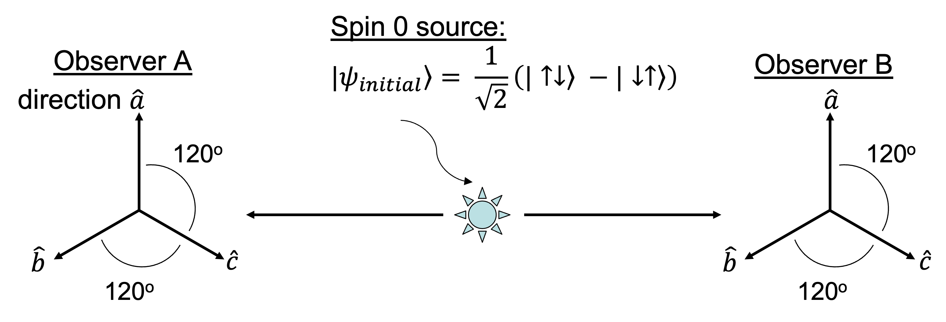
(Note: directions ($\hat{a}$, $\hat{b}$, $\hat{c}$) all lie in the plane of the page, it is easy to incorrectly misinterpret the diagram above as showing 3-D right handed coordinates)
The existence of local hidden variables would mean that each particle carries an instruction set of what would be measured along any of these three direction choices. In this experiment, with $\ket{\psi} = \frac{1}{\sqrt{2}}(\ket{+-} - \ket{-+})$, the two particles must have "opposite" instruction sets to ensure perfect anticorrelation. These hidden variables need to exist before any measurement is made and include instructions for measurements along all measurement directions.
The experiment repeats many times, and the outcome ($+$ or $-$) for each particle is recorded (but not the axis of measurement). We compute the probability after many trials that the two observers record the SAME outcome (both $+$ or both $-$). By enumerating all possibilities, we quickly establish that Prob(same) $\le$ 4/9, no matter what the distribution of "hidden instruction sets" might be. This is a Bell inequality; it arises simply from counting. It must hold for any local hidden-variable theory.
More details are found in the next section and our downloadable notes.
References: The original EPR paper is quite readable (Phys. Rev. 47, 777 (1935)), but we find the suggested experimental context of position and momentum harder for our students than the spin version. The setup we use follows Mermin's (excellent) paper "Is the moon there when nobody looks?"
The previous section on Hidden Variables set up an example of a "Bell test." An initial 2-particle state $\ket{\psi} = \frac{1}{\sqrt{2}}(\ket{+-} - \ket{-+})$ is created, and well-separated observers Alice and Bob each measure one of the two particles. They choose to measure spin along one of three randomly-selected axes, $120^{\circ}$ apart. Each individual measurement is recorded only as $+$ or $-$ (they do not record the axis measured). After many measurements, they compare outcomes and determine Probability(same outcome).
A quantum calculation begins by computing Prob($++$) in the special case that observer #1 measures in the z-direction, and observer #2 is in any of the (three) $\hat{n}$ directions:
$Prob(\#1 \ is\ +\hat{z}, \#2\ is +\hat{n}) = |\ \bra{+}\ \bra{+_n}\ \ket{\psi}\ |^2$
Using $\ket{+_n} = \cos{\theta/2}\ket{+} + \sin{\theta/2} \ket{-}$, we find this probability is $\frac{1}{2}\sin^2{\theta/2}$ (see lecture notes for more details) Adding Prob(--) = Prob(++), we get (for this situation):
Prob(same) = $\sin^2{\theta/2}$ .
Averaging over the other possibilities for measurement combinations (e.g. that $\hat{n}$ can be oriented at $\theta = 0, \pm 120^{\circ}$ with equal likelihood), we conclude Prob(same) = 0.5
This outcome has been well-tested experimentally. This violation of the "Bell inequality" (Prob(Same) $\le$ 4/9) experimentally validates quantum theory and is explicitly inconsistent with local hidden variable theories.
Reference:
"Significant-Loophole-Free Test of Bell’s Theorem with Entangled Photons ", Marissa Giustina et al., Phys. Rev. Lett. 115, 250401 (2015)
FAQs
Can I edit the materials to make them better fit my course?
Yes, please edit the materials. We do not intend for the materials to be used wholly as written. Rather, they form a complete set that a faculty member can pick and choose from as it fits their schedule, the material already taught, and the interests of both the faculty member and student.
When do I use this module in my course?
Steven Pollock teaches at research-intensive public institution and uses these materials in junior or senior-level undergraduate quantum mechanics courses, which currently all follow a spins-first curriculum (using McIntyre's Quantum Mechanics textbook.)
He teaches entanglement and EPR midway through the first semester (this is largely following McIntyre's Chapter 4 treatment)
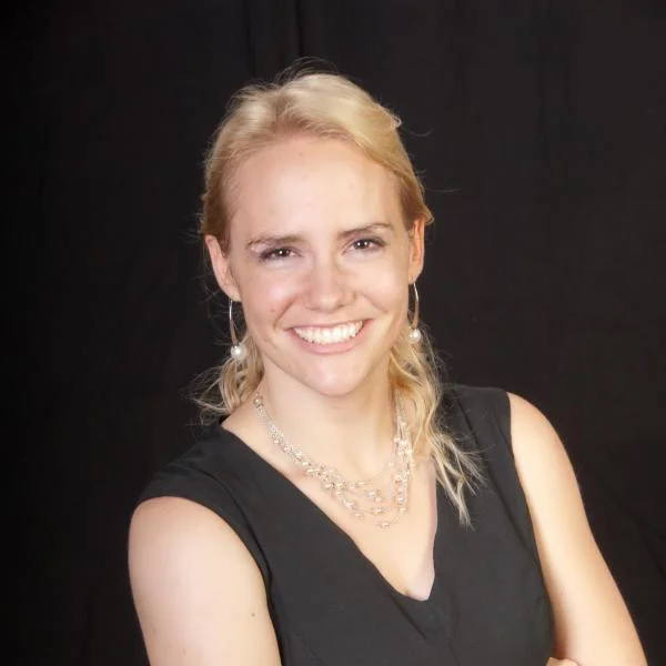
Gina Passante teaches at a primarily undergraduate, large, Hispanic-serving institution and use these materials in several of her quantum mechanics courses at the undergraduate and master's levels.
She teaches an introduction to entanglement and a conversation of "spooky action at a distance" when she teaches the "qubits, quantum gates, and teleportation" material. But the discussion about the EPR paradox and the Bell inequalities is taught at the master's level.
What if I need help implementing active learning in my class?
Physport.org has some short guides to help you facilitate in-class tutorials, as well as to help you implement clicker questions in lectures effectively.
Is there research published about using these materials?
Yes, our AJP paper gives more information on how we implement these types of materials in our upper-division classes.
Explore other topics within QIS for QM
Who we are
We are PER research faculty teaching at very different institutions - different in class sizes and setups, student demographics, institutional research-focus - but all interested in helping introduce undergraduates to basic elements of Quantum Information Science. We have all taught a variety of quantum courses for many years.
The materials you will find here are not meant to be taken as givens, this is not a "fixed curriculum" that you are supposed to fully adopt (or reject). We hope that you will be inspired by some of the activities, notes, concept-tests, homeworks and more, and will borrow and adapt them for your own situation and students. We do not all use exactly the same materials ourselves.
We have borrowed where we can from PER literature on Quantum Mechanics (and tried - but apologize up front where we occasionally have failed - to appropriately credit the the hard development work of others!) We do not claim that these materials are "Research-validated" (they are still under development), but cheerfully present sometimes half-baked or partially-tested materials that we might argue are "research-based", a vaguer but perhaps more realistic description.
We welcome feedback and suggestions. If you make significant changes or additions, and particularly if you have classroom evidence that suggests it works well - let us know. We hope someday this site will be flexible enough to allow for community-sharing of new resources, and will work towards making that happen. (See contact information below.)
 |
Gina Passante is Associate Professor of Physics and Director of the Catalyst Center for the Advancement of Research in Teaching and Learning Math and Science at Cal State University Fullerton. She received her Ph.D. in quantum computing at U. Waterloo before transitioning to PER. |
 |
Steve Pollock is a Physics professor at CU Boulder who has engaged in PER for 20+ years. He has a background in theoretical nuclear physics. He is an APS Fellow, and was named US Professor of the Year in 2013. His PER work is focused on assessment and curricular materials development in upper-division physics courses. Please email if you are interested in teaching materials for other courses (including middle division Classical Mechanics, E&M, and others). He can be reached at Steven.Pollock (at) Colorado.edu |
 |
Bethany Wilcox is a Physics professor at CU Boulder. Her PER work focuses on the development of research-based and validated assessments of student learning that can be used to measure the impact of curricular changes or compare student learning across courses and institutions. In particular, she is utilizing advanced testing theories to explore viable options for creating modular assessments that can address variations in content coverage in across courses. |
We acknowledge the hard work of our students, including Josephine Meyer (University of Colorado Boulder), Jonan-Rohi Plueger (University of Colorado Boulder), and Bianca Cervantes (former California State University, Fullerton).
We are funded in part by NSF DUE- 2012147 and 2011958: Collaborative Research: Connecting Spins-First Quantum Mechanics Instruction to Quantum Information Science
PLEASE USE AND ADAPT whatever is helpful to you, however it will most benefit your students. Please credit our work if you share your materials beyond your own classes. Please make an effort to keep assessment materials off the open web - alter questions for your students.