How do I develop student learning outcomes for physics courses?
Student learning outcomes, or SLOs, are an explicit statement of what you expect students to learn. SLOs can be defined for a topic, course or an entire program of study. This recommendation focuses primarily on course-level SLOs, as opposed to topic-levels SLOs or program-level SLOs. SLOs define what is expected of students and what it means to understand something, without defining how that understanding will be taught. SLOs help sharpen the focus on student learning, and aim the attention of students and instructors on the essential messages of the unit, course, or major. SLOs are valuable in shaping the instruction and assessment within each course, and ensuring coherence and cohesion across sections, instructors, and the curriculum. For example, an course-level SLO for a second-year physics course might be “At the end of this course, students should be able to apply conservation of energy to real-world thermal systems such as home heating” (Carl Wieman Science Education Initiative, 2009).
What is a student learning outcome (SLO)?
A student learning outcome (SLO) is a specific, measurable statement of student learning. An SLO states what a student should be able to do as a result of learning. It should be specific enough that most people could agree on what it means, and you could assess whether a student achieved the outcome. Outcomes also reflect what you value in student learning and thus target your instruction, and student effort, appropriately.
SLOs usually take the form “A student should be able to...” Course-level SLOs are quite broad, and define what the course is about; typically a course will have 5-10 SLOs (Carl Wieman Science Education Initiative, 2014). Here are some example course-level SLOs:
- A student should be able to project a given vector into components in multiple coordinate systems (Classical Mechanics).
- A student should be able to translate a physical description of an upper-division electromagnetism problem to a mathematical equation necessary to solve it. (Upper-Division Electricity and Magnetism)
- A student should be able to appreciate that physics is relevant to the real world and is a useful tool for solving problems (Introductory Physics)
- A student should be able to make a presentation quality graph showing a model and data (Introductory Physics Laboratory).
Note that each statement uses a specific, active verb (“project”, “translate”, “appreciate,” make”) which describes the type of understanding or skill that is desired.
Course-level student learning outcomes are not the same as a syllabus: A syllabus will list the topics and material that will be covered and the time that will be spent on them, whereas course-level SLOs will describe what students are expected to be able to do as a result of learning about those topics. It is recommended that SLOs be listed on the course syllabus.
Below is a list and explanation of various terminology related to student learning outcomes.
| Level | Terms (synonyms in italics) | Explanation | |
|
Program or major |
|
“At the end of the program, a graduate should be able to...” These define what a student should be able to do at the end of the entire program of study, and may be required for accreditation. |
|
|
Course |
|
“At the end of the course, a student should be able to...” These define what a student should be able to do at the end of a course, and is the focus of this expert recommendation. |
|
|
Topic or lesson |
|
“At the end of the lesson, a student should be able to...” These define what a student should be able to do at the end of a lesson, topic, or module. |
Because student learning outcomes can be at different levels of the learning process, it is useful to determine the period of time which is described by the learning outcome (e.g., course, topic, or program). Some instructors also organize their SLOs by lecture, section, or unit: You can use whatever level(s) of organization are most useful to you. All of these levels of learning outcomes should be aligned for a coherent major, and a coherent course: The topic-level SLOs should connect to the course-level SLOs, and the course-level SLOs should build towards the program-level SLOs.
Why are student learning outcomes useful?
Defining and circulating SLOs help primarily with communication -- with students and other instructors. They also help with vertical and horizontal alignment of the curriculum, course planning, and department strategy. Course-level SLOs help many people refine their understanding of the course:
- Students so that they understand expectations and organize and focus their learning.
- Instructors of that course to help them focus and design instruction and assessment, and align with others teaching the same course.
- Instructors of adjacent courses to ensure they know what students should know at the start or end of their own course.
- The department to ensure that program-level SLOs are all addressed, complement and build on each other across courses, helping to inform, assess, and shape the curriculum.
Instructors report that clear course- and topic-level SLOs make writing exams easier, and they feel that they can more easily navigate the difficulty of what to cover in the course (including the breadth vs. depth dilemma). Course- and topic-level SLOs also help support student success; by defining expectations explicitly SLOs can help level the playing field for marginalized groups, including first-generation college students and others who may not be aware of the often implicit expectations for what they need to do to succeed in a course. Students are overwhelmingly positive about having access to SLOs (Simon and Taylor 2009), finding that they help to keep them on track, focus, see the organization and relative importance of material in the course, and generally know what they need to know.
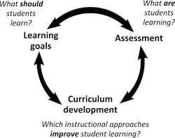
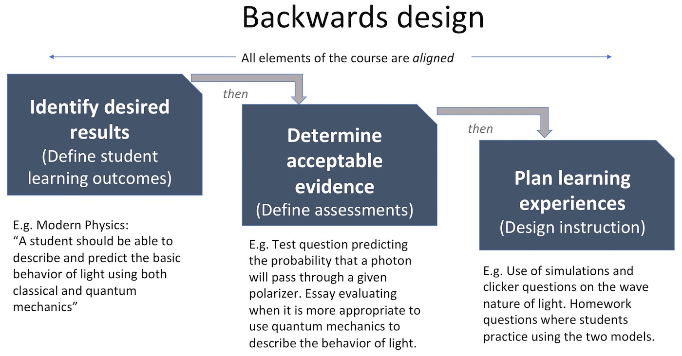
SLOs are used within a process called “backwards design”, where SLOs form the target of the instruction and the instructional planning works “backwards” from that intended end-point. What should students be able to do? What evidence would convince you of student success? How will you help students get there? (Bowen 2017) Backwards design can be used at the level of a topic, course, or program. The goal of backwards design is alignment -- alignment between goals, instruction, and assessment.
Having a departmental decision to universally adopt at least a subset of the course-level SLOs can be productive (both for course development, and sustainability). Even when course-level SLOs are defined by a department, rather than an individual instructor, there is still substantial room for individual instructors to have freedom and autonomy over how to teach their classes. Defining SLOs at any level does not dictate exactly what examples or content will be used to develop the desired skills, or how the content will be taught. Also, course-level SLOs might only cover 70-80% of the course content (Carl Wieman Science Education Initiative, 2014). Thus, course-level SLOs provide a valuable structure or scaffold for a course, guiding teaching, and ensuring a quality student experience that has been carefully designed. The instructor is still free to choose the important examples or methods for teaching the content, and to include topics that speak to their personal passion.
What is a good process for developing student learning outcomes?
Course-level SLOs can be developed by an individual faculty member for their course, or by a group of faculty aiming to reach consensus. Program-level SLOs are typically defined by a department as a whole. Finer-grained SLOs (e.g., topic, lecture) are typically defined by the faculty member(s) teaching the individual course. Faculty working groups can be incredibly valuable for developing course-level SLOs for a course or set of courses. A working group can be a faculty learning community or departmental team, composed of those who have previously taught the course and teach adjacent courses. Such meetings often provide a valuable forum for deep and productive conversations among faculty about student learning, attitudes, and the major. For example, at University of Colorado Boulder faculty wrestled with the question of how many times a student might need to see a particular topic, or how it would affect student attitudes for Math Methods to be the first upper-division course they take in the major (Pepper et al. 2011). It is helpful to have a facilitator set the agenda, take notes, review and synthesize materials and facilitate consensus. For guidance on facilitating such discussions, and prompting questions for faculty, see the short handout Facilitating Learning Goal Discussions (Chasteen, 2018). For a useful, short discussion of developing consensus course-level SLOs at University of Colorado Boulder, and lessons learned, see Pepper et al. (2011).
Even if not working with a faculty group, individual faculty should talk to their colleagues about their course-level SLOs; your course is part of a working whole, not an isolated independent unit. This is particularly true of some courses (e.g., if the course is a fundamental prerequisite to other courses or part of a two-course sequence), but all courses play a role in fulfilling the mission of a department and other faculty will have relevant expertise and guidance to provide. New faculty in particular should consult with senior colleagues and departmental guidelines.
- Start with the simple question, “What should students get out of this course?”
- Use the “prompts and probes” below to help you think about the course.
- Consider looking at IUB’s “Decoding the Disciplines” page that describes student “bottlenecks”.
- Review example SLOs and adapt them for your needs (see examples below).
- Review previous exams in the course and work backwards from there. What was this exam question testing? What might be the related SLO? What is missing?
- Talk to faculty who have taught that course, or adjacent courses. What do they think is important to teach? What do students often not learn? What did instructors of subsequent courses expect students would be able to do that they were not?
- Show your SLOs to faculty and students to identify terms that lack clarity or precision.
- Plan to review and revise the SLOs over time.
- What is this course about?
- What are the big ideas that you want to get across in this course?
- How is this course different from course X (higher/lower level course)?
- What is this course’s place and role in the curriculum overall? Who takes it, and what do they need?
- If you were writing a letter of recommendation for a student who just completed this course, what would you like to be able to say that they can do? What will they know and what will they value?
- Are there topics in the course where students really seem to struggle (“bottlenecks”) ? How do you know that they struggle?
- Do you have other goals beyond the content/knowledge goals, such as critical thinking, attitudes, beliefs, or increasing student interest in the major? (Giving examples can be useful.)
- What knowledge and skills are the students expected to have for a follow-on course (if applicable)? What do they typically lack when entering that follow-on course?
- After you lecture on topic X, what do you expect a student to be able to do?
- If a student gets this exam question right (wrong), what does it show they can (can’t) do?
- What do you mean by “understand”?
- How might you measure that type of student learning?
How do I write appropriate student learning outcomes for different levels of courses?
Course-level SLOs will look different for different levels of courses, because the students and your expectations of those students will be different.
Courses across the curriculum should have learning outcomes that cover a range of levels of cognitive complexity (e.g., Bloom’s Taxonomy; see next section), from simple memorization to critical thinking skills. It is not the case that lower-division courses should only have lower-level SLOs, and upper-division courses should only have higher-level SLOs. Upper-division courses still require students to memorize terminology (lower-level SLO), and lower-division courses should require creative problem solving (higher-level SLO). However, upper-division courses are likely to have a greater focus on higher-level SLOs, including critical thinking, creative solutions, and independent work. Because upper-division students have a broader foundation of knowledge and skill, upper-division courses can build on that previous knowledge and their commitment to the discipline to develop these high-level skills and understandings. And while lower-division courses may require students to develop initial awareness of ideas or start to develop skills, in upper-division courses the expectations may be that students develop a level of mastery in the same topics or skills. For examples of upper-division course-level SLOs, see the section on examples below.
Upper-division course outcomes are also part of a greater whole, in that they are part of a cohesive curriculum which is developing students as experts in the discipline. Thus, if the program has program-level learning outcomes (PLOs), upper-division course-level SLOs must build towards those program-level SLOs in conjunction with other courses. This is true of all courses in the major. Upper-division course-level SLOs are thus less independent from the SLOs in other courses than might be the case in the lower-division. As such, there is also likely to be greater departmental interest and concern in developing upper-division course-level SLOs.
How do course-level student learning outcomes relate to learning a particular topic?
Instruction and assessment about specific topics (for example, Newton’s Third Law) should be guided by the course-level SLOs. It can be helpful to start with course-level SLOs, but you may eventually want to define topic-level SLOs to help design instruction and assessment at a finer-grained level. Typically, there might be 2-5 topic-level SLOs for a particular topic.
| Example course-level SLO (5-10 per course) | Example aligned topic-level SLOs (2-5 per topic; each below is from a distinct topic or lesson) |
|
A student should be able to describe and predict the basic behavior of light using both classical and quantum mechanics. |
A student should be able to:
|
You can see more examples of course- and topic-level SLOs in the section on examples below. While course-level SLOs often need to be indirectly assessed through multiple forms of assessment (such as several exams and homework questions), topic-level SLOs can more often be directly assessed through specific exam question(s) or other assessments.
A valuable resource for developing topic-level SLOs is the Decoding the Disciplines approach which identifies student bottlenecks in learning, and unpacks the mental processes necessary for overcoming these bottlenecks. You can also view a short video on the decoding process here.
How do I write good student learning outcomes?
Not all SLOs are created equal. SLOs will be more useful if you write them well because then they will be more helpful in guiding instruction and assessment. This takes time and is usually hard to hit on the first try. This is also an opportunity to be choosy -- take this opportunity to streamline the course and keep it focused on the core ideas.
Course-level SLOs describe what is important in your course. What would you be mortified to discover your students hadn’t taken away from your course? These are your top outcomes. Below is a checklist you can use when writing, and revising, a course- or topic-level SLO (adapted from Carl Wieman Science Education Initiative, 2014). Write these SLOs about what the student should be able to do, using well-defined verbs that appropriately describe the level and type of understanding that is desired. Make them clear, and measurable. Use everyday language when possible.
Checklist for developing clear student learning outcomes (SLOs)
- Does the SLO identify what a student should be able to do after the course or topic is completed?
- Is it clear how you might test achievement of the SLO?
- Do the verbs have a clear meaning? (e.g., avoid the use of the words “understand” or “know”)
- Is the SLO aligned with the level of cognitive understanding expected of students? (i.e., higher- or lower-level understanding)
- Do the SLOs cover the range of types of desired understanding?
- Is the SLO written in a way that students will understand it?
- Is it possible to write the SLO so it is relevant and useful to students?
Write SLOs at a variety of cognitive levels
Some outcomes are lower cognitive levels, such as asking students to recognize a term, or state a definition in their own words, or choose the right variable from a list. Others are at a higher cognitive level, such as asking students to analyze and graph data, evaluate the suitability of different methods for solving a problem, or design an experiment. A useful tool for evaluating cognitive difficulty is Bloom’s Taxonomy (Bloom 1956), which describes different cognitive levels from “remember” through “create.” While there are some critiques of Bloom’s Taxonomy because learning is not actually a hierarchical and linear process (Berger 2018), it is still a useful tool for considering the level you are trying to get your students to achieve.
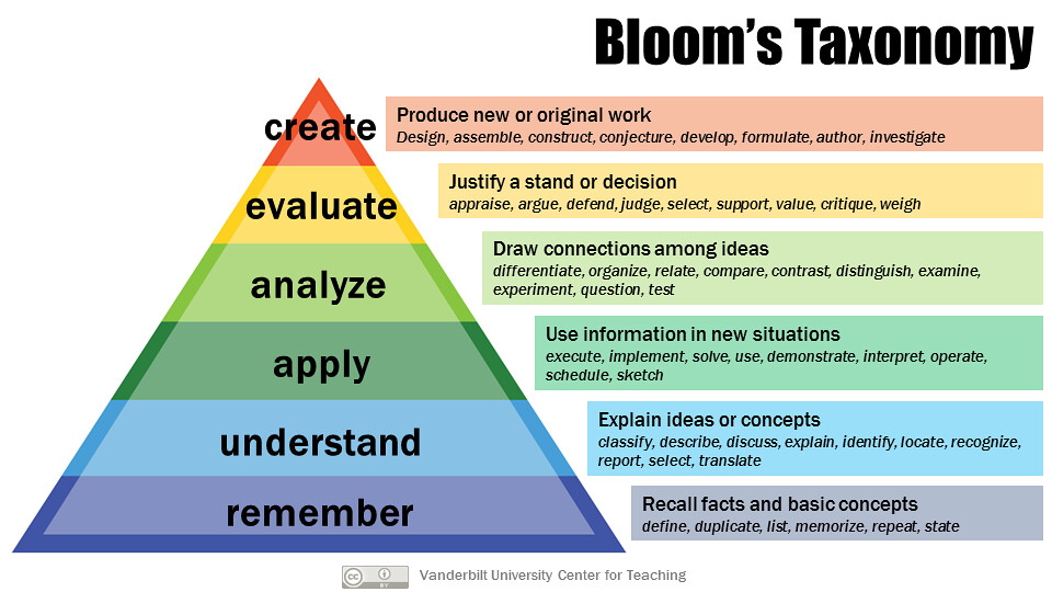
Bloom’s Taxonomy, courtesy of Vanderbilt University Center for Teaching CC-BY
Start SLOs with a clear, measurable verb
Each SLO uses a specific verb to communicate the expectations of students; see Bloom’s Taxonomy figure above for ideas of such specific verbs. A common mistake with developing SLOs is to write that students should “understand” or “know” something. These verbs are too vague to serve the purpose of clear communication or to drive assessment. Use more specific, measurable language. One of the reasons I use Bloom’s Taxonomy for writing learning outcomes is because many people have developed useful lists of verbs and assessment practices that align with different levels of Bloom’s (my favorite is here). A look through some of these lists can help you find more specific verbs -- for example, if you know that you want your students to “understand Newton’s Laws” (which is too vague), what you want instead is for them to be able to “solve a problem using Newton’s Third Law.” Or at a lower level, perhaps you want them to “summarize Newton’s Laws in their own words.” Or, at a higher level, “students will be able to defend the choice of Newton’s Third Law as a solution method for a given problem.” Any of these new formulations lead more clearly to instruction and assessment; they are more measurable.
Use SLOs that cover a range of desired student behaviors
While many SLOs are written in terms of cognitive learning (e.g., facts and concepts), this is only one type of outcome you might be interested in. Below are some other types of learning outcomes to consider. (Phys21, Gagne, 1985)
|
Type of outcome |
Description |
Example |
|
Cognition |
Physics-specific knowledge, facts and concepts; terminology, details, classifications, principles. |
A student should be able to summarize Newton’s Laws in their own words. |
|
Procedures and skills |
Techniques, methods, problem solving, experimental skills. |
A student should be able to perform appropriate statistical analysis of data. |
|
Metacognitive abilities (expert learning) |
Self-awareness of what helps them learn, studying and learning strategies. |
A student should be able to identify which areas of the course cause them the most difficulty, and which are most intriguing. |
|
Professional skills |
Communication, career opportunities, interview skills. |
A student should be able to give an articulate oral presentation on the topic. |
|
Attitudes and beliefs |
Appreciation, enjoyment, value, habits of mind. |
A student should be able to recognize that the world is not mysterious and unpredictable, but is governed by natural laws. |
How can I assess student learning outcomes?
Any SLO should be directly or indirectly measurable. How would you know if a student had achieved that SLO? Course-level SLOs may be measurable on a quiz, homework, test, project, lab, survey, oral exam, and more. Outcomes can be assessed formatively and summatively (i.e., during learning, or at the end to determine if learning has occurred). An outcome that asks whether students appreciate physics, or feel confident that they can do physics might be assessed on a feedback survey or a personal essay, for example. Because course-level SLOs are quite broad, you might need more than one assessment to convince you whether a student has achieved a particular SLO. Topic-level SLOs are often more specific and thus directly measured with a single assessment. The topic of assessment is beyond the scope of this expert recommendation, but you can find relevant learning assessments in PhysPort’s assessment database.
I have my student learning outcomes. Now what?
Once you have developed course-level SLOs, you can use the process of backwards design to use them to direct instruction and assessment. (Bowen 2017) For each SLO, outline the types of assessments you might use, and develop instructional techniques. Here are specific times you might use or refer to your course- or topic-level SLOs:
- Use them when designing the course as a whole. See the Backwards Design Template from Vanderbilt (Bowen 2017) for useful support for this process.
- List them on your syllabus to orient students to your goals.
- List relevant SLOs at the start and end of each day’s class, as well as on assignments, handouts, and study guides.
- Review them when writing your lecture and class activities for the day.
- Review them when writing your exams and other assessments. Are you assessing the right outcomes, and at the right level? Consider identifying the Bloom’s level of each exam item, called “Blooming” your exam. (Crowe, Dirks, and Wenderoth 2008)
- Share with faculty teaching the adjacent courses.
How do student learning outcomes relate to the program or the major as a whole?
Program-level SLOs are learning outcomes written at the level of the entire major or program. The course-level SLOs should collectively align with and build towards the program-level SLOs. For example, program-level SLOs might include (Phys21):
- Upon completion of the program, students should be able to represent basic physics concepts in multiple ways.
- Upon completion of the program, students should be able to solve complex, ambiguous problems in real-world contexts.
- Upon completion of the program, students should demonstrate critical professional and life skills.
The report Phys21: Preparing Physics Students for 21st-Century Careers (Chapter 4) includes lists of possible program-level SLOs appropriate to prepare students for diverse careers. These are available in the examples below. Course-level SLOs must then build students’ capacity in the areas of these program-level SLOs.
Both program-level and course-level SLOs are usually required by institutions and accreditors. Accreditors typically require program-level SLOs to be posted on program web sites and course-level SLOs to be included in all course syllabi. Program-level SLOs are required to be assessed on a fixed timetable, usually every 3-5 years for a complete cycle of assessment. Required assessment of program-level SLOs can be used as a key element of internal departmental processes to improve your programs. Creating course-level SLOs is a great way to ensure that the work required to define program-level SLOs is actually useful for the department in designing a coherent and rigorous curriculum. Defining program- and course-level SLOs also supports a more intentional and coherent major. The process of aligning program- or course-level SLOs is called “curricular alignment” or “curriculum mapping”, and is usually done by listing out the program-level SLOs, and then identifying (in a large table) which course(s) should address those program-level SLOs through their course-level SLOs. Through this process, some departments have found that concepts were repeated from course to course, or critical ideas were omitted entirely from the curriculum. You can find more about that process from the CU-Boulder handout on curricular alignment and the SERC guide to Building Strong Departments.
Where can I find more information?
- CIRTL Massive Open Online Course (MOOC) “An Introduction to Evidence-Based Undergraduate STEM Teaching: Learning Objectives”. A series of short videos on topic-level SLOs including “Why do we need learning objectives,” “Introduction to backwards design”, “Course scale goals vs. topic level objectives” and “What does it mean to know something”.
- Decoding the Disciplines. This page describes how to unpack expert understanding of a topic, allowing formulation of student learning outcomes that overcome common learning challenges (“bottlenecks”).
- Vanderbilt Backwards Design template. This page provides a useful overview of backwards design, along with a downloadable template for course planning using this approach.
- Carl Wieman Science Education Initiative Learning Goals Page. This page has a variety of learning outcome resources including guidance, articles, and example outcomes.
- Phys21: Preparing Physics Students for 21st-Century Careers. Chapter 4 of this report includes lists of possible program-level SLOs appropriate to prepare students for diverse careers. Many are very suggestive of course-level SLOs.
- Building strong departments. This geoscience education page at the Science Education Resource Center (SERC) has very useful and relevant articles and ideas for setting department vision, program level SLOs, program assessment, and curricular alignment.
- NILOA: National Institute for Learning Outcomes Assessment. An organization with resources to support the development of learning outcomes, including A Brief Guide to Creating Learning Outcomes.
What are some example student learning outcomes?
It is very useful to start with example SLOs as you work to draft your own. Below we provide some example SLOs developed from other sources. It is typical to have 4-6 program-level SLOs and 5-10 course-level SLOs for each course, but these numbers, and the organization of the SLOs, will vary by instructor preference. Many of the examples below are more detailed than typical, so keep in mind that you don’t need to aspire to this level of detail for your own department. In addition, this is not meant to be an exhaustive list.
Reprinted from Phys21 Learning Goals to Support Diverse Career Directions (Phys21: Preparing Physics Students for 21st-Century Careers, Chapter 4). Copyright American Physical Society CC-BY
Recommended learning goals for undergraduate physics programs: Upon completing an undergraduate physics program, ideally a graduate should be able to:
A. Physics-Specific Knowledge
- Demonstrate the ability to apply fundamental, crosscutting themes in physics, including conservation laws, symmetry, systems, models and their limitations, the particulate nature of matter, waves, interactions, and fields.
- Demonstrate competency in applying basic laws of physics in classical and quantum mechanics, electricity and magnetism, thermodynamics and statistical mechanics and special relativity, and the applications of these laws in areas such as optics, condensed matter physics, and properties of materials.
- Represent basic physics concepts in multiple ways, including mathematically (including through estimations), conceptually, verbally, pictorially, computationally, by simulation, and experimentally.
- Solve problems that involve multiple areas of physics.
- Solve multidisciplinary problems that link physics with other disciplines.
- Demonstrate knowledge of how basic physics concepts are applied in modern technology and apply this knowledge to the solution of applied problems.
B. Scientific and Technical Skills
- Solve complex, ambiguous problems in real-world contexts.
- Define and formulate the question or problem, i.e., ask the right question.
- Perform literature studies (print and online) to determine what is known about the problem and its context by locating, reading, analyzing, evaluating, interpreting, and citing technical articles; manage scientific and engineering information so that it is actionable.
- Perform trade studies [52] to identify the optimum technical solutions among a set of proposed viable solutions, based on applied experience.
- Identify appropriate approaches to the question or problem, such as performing an experiment, performing a simulation, developing an analytical model, and making rough estimates based on specific strategies.
- Develop one or more strategies to solve the problem and iteratively refine the approach.
- Design an appropriate experiment or simulation to address the problem, taking into account precision, repeatability, and signal-to-noise ratio.
- Engage in appropriate statistical analysis of results.
- Identify resource needs for solving the problem and make decisions or recommendations for beginning or continuing a project based on the balance between opportunity cost and progress made.
- Show how results obtained relate to the original problem, determine follow-on investigations, and place the results in a larger perspective.
- Demonstrate instrumentation competency: competency in basic experimental technologies, including vacuum, electronics, optics, sensors, and data acquisition equipment. This includes basic experimental instrumentation abilities, such as knowing equipment limitations; understanding and using manuals and specifications; building, assembling, integrating, operating, troubleshooting, and repairing equipment; establishing interfaces between apparatus and computers; and calibrating laboratory instrumentation and equipment.
- Use basic hand tools.
- Interface apparatus to computers using tools such as LabVIEW, MatLab interface modules, and GBIP.
- Use laboratory tools such as oscilloscopes, sensors, electronics, optics, vacuum systems, materials fabrication tools, signal digitizers, and signal analyzers.
- Make effective use of advanced analytical or process tools.
- Demonstrate software competency: competency in learning and using industry-standard computational, design, analysis, and simulation software, and documenting the results obtained for a computation or design. Examples include:
- General-purpose computational tools: Excel, MatLab, Mathematica, Maple
- Optical computational tools: OpticStudio, CODE V, OSLO, TFCalc
- Electrical computational tools: SPICE, PSPICE
- Mechanical computational tools: SOLIDWORKS, Pro/ENGINEER B.4.e. Physics computational tools: COMSOL Multiphysics
- Educational simulation tools: Physlets, PhET Simulations
- Demonstrate coding competency: competency in writing and executing software programs using a current software language to explore, simulate, or model physical phenomena.
- Demonstrate data analytics competency: competency in analyzing data, including with statistical and uncertainty analysis; distinguishing between models; and presenting those results with appropriate tables and charts.
C. Communication Skills
- Communicate with many different audiences from many different cultures and scientific backgrounds, understand each audience and its needs, and make the communication relevant and maximally impactful for that audience.
- Obtain information and evaluate its accuracy and relevance through reading (print and online), listening, and discussing.
- Articulate one’s own state of understanding and be persuasive in communicating the worth of one’s own ideas and those of others.
- Communicate in writing about scientific and technical concepts concisely and completely, and revise writing to achieve grammatically-correct and logically-constructed arguments.
- Organize and communicate ideas using words, mathematical equations, tables, graphs, pictures, animations, diagrams, and other visualization tools.
- Teach a complex idea or method to others, use feedback to evaluate the learning achieved, and develop revised strategies for improved learning.
D. Professional/Workplace Skills
- Work collegially and collaboratively in diverse, interdisciplinary teams both as a leader and as a member in pursuing a common goal.
- Identify independently what must be understood, and learn it.
- Generate new ideas.
- Obtain knowledge about existing technology resources relevant for the task at hand. For example: How is the technology made? How does it work? What does it cost? Who tests it? What industries are affected by it? Where are the centers of these industries located? Where can the computational resources needed for the task be found? Which companies make the instrument needed for the experiment, and how do their products differ?
- Demonstrate familiarity with basic workplace concepts. Examples include:
- Program and project management, including planning, scheduling, tracking progress, adapting, and working within constraints
- Budgeting and financial management
- Quality assessment and assurance
- Legal, regulatory, and ethical issues; compliance, intellectual property, and employment law, including issues of workplace behavior with regard to gender, race, sexual orientation, disability, etc.
- Effective management of difficult situations, including poor team performers, K-12 classrooms, irate customers, etc. D.5.f. Safety; working with and enhancing the safety culture in the workplace
- Display awareness of regional and national career opportunities and pathways for physics graduates.
- Demonstrate awareness of standard practices for effective résumés and job interviews, as well as professional appearance and behavior. Examples include:
- Assessment of one’s skill set and its relevance to the job
- Assessment of one’s strengths and weaknesses
- Interview preparation
- Appropriate and effective interview behavior, including appropriate attire and personal grooming
- Maintaining an informative professional online presence through LinkedIn, etc.
- Demonstrate critical professional and life skills, including completing work on time, optimism, realism, time management, responsibility, respect, commitment, perseverance, independence, resourcefulness, integrity, ethical behavior, and cultural and social competence.
Adapted from UBC Phys100 goals (Good Examples of Learning Goals at UBC and CU)
- Apply conservation of energy and thermal physics principles to real-world thermal systems, such as home heating and climate change.
- Apply knowledge of work and Newton's laws to calculate basic dynamics and energy consumption of common transportation systems (cars, bicycles etc.)
- Qualitatively explain how electricity is generated in various types of power plants and the --life cycle‖ of electricity from production through transmission to consumption, and calculate power consumption for various common circuits.
- Use algebra to solve simple equations.
- Appreciate that physics is relevant to the real world and is a useful tool for solving problems.
- Develop the inclination and ability to apply problem solving techniques to simplify "real world" problems in terms of simple physics concepts and to compute or estimate solutions.
- Recognize that scientific conclusions - whether from an outside source or from your own calculations - may be incorrect, and develop the ability to check these conclusions with simple calculations, 3rd party information, and/or common sense.
Week 1. Introduction, Course Outline, discussion of techniques, Measurement, Units, Data Analysis, Experimental Error
A student should be able to:
- appreciate why active engagement techniques are being used in this class
- access the course website to find more information
- summarize the expectations for course content and student workload
- apply their knowledge of measurement error to determine what an appropriate number of sig. figures is for a particular measurement device
- describe in simple terms the general nature of a scientific theory and its relationship to the experimental data
- explain the nature of a scientific model
- use and convert between various units
Week 2. Intro to Conservation Laws, Conservation of Energy, Dynamic Equilibrium
A student should be able to:
- identify correct system boundaries needed to apply conservation laws
- explain how energy can remain at a constant level even when there is a flux of energy into or out of the system
- give examples of a physical system in dynamic equilibrium
- calculate kinetic and potential energies in mechanical systems
- recognize assumptions needed to apply conservation of mechanical energy
- explain the effect of friction and air drag on the energy of a mechanical system
Week 13. Electricity Generation and Distribution, and Environmental Impacts
A student should be able to:
- compare the cost of electricity and GHG production for various forms of power generation systems (hydro, wind, coal, nuclear, solar)
- discuss the advantages and disadvantages of these power generation systems
- calculate power losses in electricity transmission lines and explain why we use high voltage transmission lines
- estimate the energy available in wind, hydro and fossil fuels.
- discuss the energy transformations for various forms of power generation systems (hydro, wind, coal, solar)
A. Consensus Themes (not SLOs)
- Students should come away with a positive attitude about experimental physics.
- Students should understand that physics is an experimental science.
- Students should have a set-like vs a point-like understanding of measurements and uncertainty. (understand mean, stdev, distributions)
- Communication of scientific process and result (especially using graphs and oral argumentation) is important.
- Learning how to write lab reports and notebooks is not a goal for the course.
- Experimental design is not a goal for the course, but small design components (or experimental choices) could be added in the later stages of the course.
- Students should not be allowed to choose their own experiments and all students in the room should be doing the same experiments.
- Any implementation should recognize the limitations of the skills/time of the TAs.
- The new course should be sustainable even when many different faculty members rotate though the course.
- This course must remain an “experimental experience” to satisfy ABET accreditation.
- The physics topics covered in the lab should include material from both PHYS 1110 and PHYS1120 (the introductory physics sequence).
B. Consensus Learning Goals and Assessment Instruments
- Students’ epistemology (i.e., theory of the nature of physics knowledge) of experimental physics should align with the expert view
- Alternative Definition: Student’s beliefs about the nature of experimental physics should align with expert physicists. This includes understanding that physics is an experimental science, what makes for a valid measurement, and how knowledge is gained through experiments.
- Assessment: Colorado Learning Attitudes about Science Survey for Experimental Physics (E-CLASS) epistemology items
- Students should have a positive attitude about the course
- Assessments: Student course evaluations (FCQ’s) with additional tailored questions
- Students should have a positive attitude about experimental physics
- Assessments: E-CLASS affect items + new questions about exp. physics
- Students should be able to make a presentation quality graph showing a model and data
- Assessments: course artifacts
- Students should demonstrate a set-like reasoning when evaluating measurements
- Alternative Definition: Students should understand that a measurement has an associated uncertainty and is not the “true” value. They should understand that repeated measurements form a distribution with a mean and a standard deviation.
- Assessment: Physics Measurement Questionnaire (validated assessment developed at Cape Town)
- Possible sub-goals for this SLO:
- Low-level of achievement
- Compute mean
- Compute standard deviation
- Understand that there is inherent distribution when measuring
- Count significant figures
- Report results properly (mean +- sig/sqrt(N) with proper significant figures
- Know when there is discrepancy between two results
- Medium-level of achievement
- Understand what sigma means
- Understand the difference between Sigma vs. Sigma/sqrt(N)
- Know how to treat outliers and when to remove data
- High level of achievement
- Propagate error
- Understand the difference between systematic vs. statistical uncertainty
- Know how to reduce systematic uncertainty – choosing the right measurement to improve, proposing causes
- Low-level of achievement
C. Additional guiding principles (things that are not our expectations of students)
- Students will not write full formal lab reports.
- Students will not choose which experiments they do each week.
- Students will not be required to learn the details of coding in Mathematica, Matlab, etc.
- Students will not be required to learn to derive differential propagation of errors formalism.
- Students will be required to put in effort appropriate for a one-credit course, which includes no more than three hours outside of scheduled class time.
From lab #1 (“skills”)
After completing this lab, you should be able to:
- Use OneNote on your tablet computer as a digital lab notebook.
- Embed an Excel spreadsheet into your OneNote notebook.
- Turn in your lab notebook to Canvas at the end of the lab for credit.
- Recognize some of the lab equipment to be used in PHYS 1140.
From Lab #2 (“skills”)
After completing this week’s lab, you should be able to:
- Create a plot using Excel that includes labels, a trendline, and a caption.
From Lab #3 (“skills”)
After completing this week’s lab, you should be able to:
- Describe how the number of measurements affects the values calculated for standard deviation (σx) and standard deviation of the mean (σxbar)
- Explain the difference between (σx) and (σxbar) and how to use each when reporting measurements.
- Decide how well two data sets agree with each other using x and σx from each set.
From lab #4 (Mechanics)
This week’s lab reinforces the learning goals of statistics of Lab 3. In addition, after completing this lab, you should be able to:
- Decide whether to use the standard deviation, σx, or the standard error of the mean, σxbar, when comparing measurements.
- Decide if two measurements likely agree with one another.
- Report a measurement using the proper number of significant figures and value for the uncertainty.
From lab #5 (Mechanics)
This week’s lab reinforces the learning goals of Labs 3 and 4. In particular, we are emphasizing:
- Understanding what σx means for the probability of a single measurement of x.
- Deciding when to use σx versus when to use σxbar.
From lab #6 (Mechanics)
After completing this lab, you should be able to:
- Use the uncertainty in a measured quantity to determine the uncertainty in a calculated quantity.
- Propagate uncertainty in two different ways.
From lab #7 (E&M)
After completing this lab, you should be able to:
- Identify and address a systematic effect.
- Modify the physical model to take a systematic effect into account.
From lab #8 (E&M)
After completing this lab, you should be able to:
- Explain the operating principles of a capacitive sensor.
- Use the results of a linear fit to make predictions.
From lab #9 (E&M)
After completing this week’s lab, you should be able to:
- Calibrate an LED/photodetector system to produce any specific color
From lab #10 (Optics)
After completing this lab, you should be able to:
- Compare measurements to determine the probability of agreement
- Make decisions about whether two sets of data represent the same underlying distribution
From lab #11 (Optics)
After completing this lab, you should be able to:
- Make a plot showing multiple data series together
- Linearize data to perform a linear fit and extract a parameter’s value
From lab #12 (Optics)
After completing this week’s lab, you should be able to:
- Determine the best colors and filters for transmitting and detecting single-frequency signals through an optical fiber.
- Transmit and demultiplex multiple audio signals through an optical fiber.
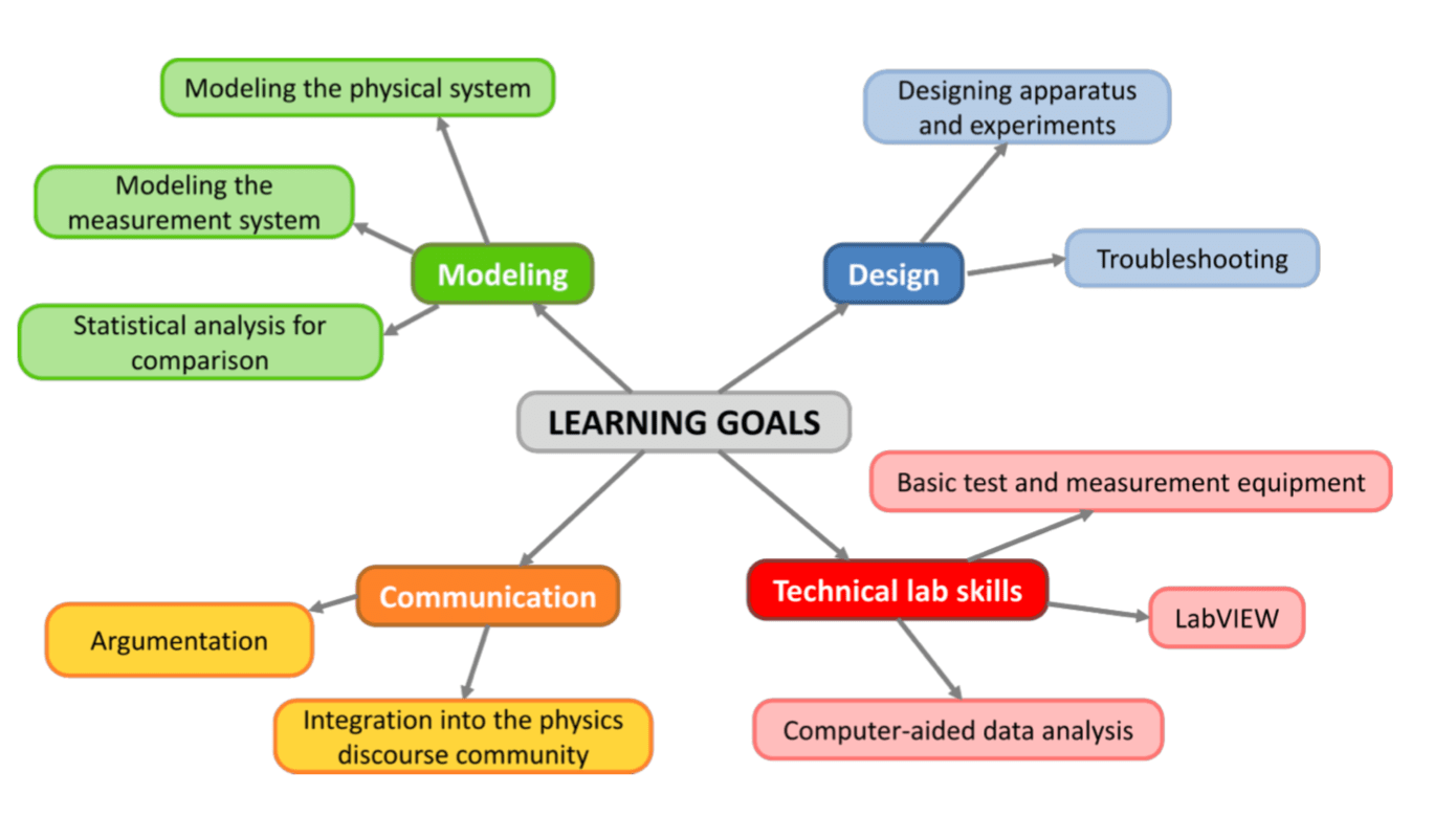
Reproduced from CU Boulder goals (Zwickl, Finkelstein, and Lewandowski, 2013), with the permission of the American Association of Physics Teachers.
Student learning outcomes for this course are organized by four main categories: Modeling, design, communication, and technical lab skills, as per the diagram below. The SLOs are organized by these categories rather than by course-level and topic-level. These four categories are somewhat analogous to course-level SLOs.
Modeling
Modeling the physical system
- Understanding the main physics ideas
- Identify the system, interactions, and environment.
- Identify the fundamental principles that are used to build the model.
- Identify the simplifying assumptions. What is being ignored?
- Developing a predictive model
- Use the main physics ideas to develop a predictive model. In general, this step is optional in the lab context because lecture courses provide opportunities for model development.
- Use words, diagrams, graphs, and mathematics to communicate the model.
- Write a mathematical expressions for the model
- For any mathematical symbols, be able to describe the physical meaning (constants, operators, variable), including how they are measured and the appropriate units.
- Using a predictive model
- Use computational and/or analytic representations of the predictive model to generate anticipated results before conducting the experiment.
- Justify the choice of all model parameters as reasonable for the system being modeled.
- Make predictions that can be compared with data as it is acquired during the experiment.
- Use the predictive model to perform a fit of the data.
- Articulating the limitations of the model
- Identify all the relevant model limitations including idealizations in the specific details (e.g., a point particle, massless string) and approximations in the fundamental principles (e.g., Newtonian vs relativistic mechanics).
- Identify what ratio of quantities must be small in order for the simplification to be valid.
- Quantitatively check, by measurement if necessary, that the system parameters are in a regime where the simplifications are valid.
- Revision of models If a prediction with measurements shows the model is inadequate to predict the data
- Generalize the predictive model to include missing elements that were intentionally or unintentionally omitted. This may require computational modeling, or approximation techniques to include the previously neglected effect.
- Redesign the physical system so that a particular simplification is valid.
- Compare the above two options and decide the better course of action based on which is more feasible, efficient, or will better answer the scientific research question.
Statistical analysis for comparison
Statistical analysis, broadly speaking, has two uses. The first is to estimate the quality of the measured data, especially, how reproducible is the data in question. The second is to compare the measured data with the predictions from a model.
- Estimating the quality of data
- Estimate the uncertainty in measured quantities.
- Describe how the uncertainty was estimated and justify what that approach gives a reliable estimate of the uncertainty (e.g., theoretical estimate from counting statistics, from repeated measurements, from the resolution of the measurement tools)
- Decide if the uncertainty changes throughout the experiment, and if it does, estimate it appropriately.
- Quantitatively describe how the measurement uncertainty could be improved with multiple measurements, i.e., if I wanted to improve my accuracy to , then I would need to average trials.
- Estimate uncertainty in derived quantities.
- Calculate the propagated error in derived quantities.
- Use error propagation to identify the largest sources of error in the experiment.
- Represent uncertainty…
- Graphically as error bars.
- Graphically, as a distribution of results like a histogram.
- Numerically using appropriate significant digits.
- Distinguish between systematic and random error sources in the measured data or derived quantities.
- Estimate the uncertainty in measured quantities.
- Understanding the methods of statistics. Given a particular statistical method (calculating an average, doing a nonlinear least-squares fit, a chi-square test)
- Explain why the method is used, what information it gives, and how it is interpreted.
- Explain the rules for carrying out the method.
- Give examples of the typical kind of data to use the method for.
- Use the method to analyze and interpret actual data.
- Comparison of data with predictions
- Decide. Students should be able to develop a list of options for comparing measurements and predictions (e.g., is it best to predict the raw data? process data so it is easier to compare with a general theory or compare across experiments? Is there a standard in the field?)
- Appraise a list of the relative merits of the options and defend a particular choice for presenting the analysis.
- Graphical. Making plots of theoretical predictions and data with correct labels, legends, and annotations.
- Use fits based on a model
- Obtain best fit parameters.
- Obtain errors in best fit parameters.
- Interpret errors in best fit parameters.
- Compare the fit with expectation to determine if the best fit is likely converged to the optimal set of fit parameters (particularly important for nonlinear model fitting).
- Plot residuals and use the plot to determine the presence of systematic error sources.
- Compare the size of the residuals to the estimated random error in the measurements.
- Chi-square: Compare the measured data and predictions using chi-square to estimate the likelihood of a discrepancy being due to random fluctuations, or something else.
- Students should be able to explain why chi-square<<1 indicates that the uncertainty has probably been overestimated.
- Decide. Students should be able to develop a list of options for comparing measurements and predictions (e.g., is it best to predict the raw data? process data so it is easier to compare with a general theory or compare across experiments? Is there a standard in the field?)
Design
Designing apparatus and experiments and carrying out experiments
A complete experiment includes all that is in the modeling category: making prediction, taking measurements, and doing a comparison. In addition, it adds aspects related to a broader view of scientific inquiry, engineering design, and troubleshooting technical problems in the lab. There are also key metacognitive strategies that are valuable when carrying out an experiment.
- “Testable research questions”
- Write a well-defined testable research question that
- specifies the independent, dependent, and control variables.
- And sufficiently operationalizes all variables so that they can be measured.
- Example:
- General question: “How does the shape of the aperture affect the diffraction pattern?”
- Testable research question: “How does the width of a parallel slit affect the 1D intensity distribution in the diffraction pattern.”
- Wise design
- Explain how the experiment that they design and carry out can be used to answer the testable research question.
- Describe other experiments that could perform a similar test and justify why this one is most appropriate.
- Use predictions about the physical system to set requirements for the apparatus (e.g., resolution, noise, and dynamic range of the measurement tools.)
- Use the requirements as design goals for the apparatus and experiment. Don’t overshoot the requirements unless it is extremely easy to accomplish.
- Evaluate practical and/or efficiency considerations and use them to constrain the design.
- Given any particular setting in the experiment (e.g., sample rate, gain setting, length of interferometer arms) students should be able to defend their choice as better or why it is one of a range of equally reasonable settings.
- In general student should be in the habit of asking and answering the following questions:
- Is that experiment/apparatus good enough?
- What counts as “good enough”?
- How can I tell if my system is good enough (short of running the whole experiment)?
- Calibration. Students should be able to define a model of the measurement system and take measurements in a simple test case to evaluate the model, and perhaps refine it. This process is usually called “calibration”.
- The quick check. Continually be in the habit of doing a “quick check” experiment prior to taking a long set of data, so that they can be sure the apparatus is working as expected and it is worth taking the time for the data.
- Plotting of data. Students should plot data during the experimental setup in order to continually compare with predictions and evaluate the data.
- Lab notebooks
- Students will use their lab notebook to record their thinking
- At the start of each day to set an agenda and plan for the day’s activities.
- While they are solving problems, debugging, modifying their setup, designing apparatus
- At the end of the day to summarize key results and a to-do list for next time and a list of unanswered questions.
- Students will use their lab notebook to record the following kinds of things.
- Diagrams of the setup
- Relevant settings on equipment.
- Location of saved data
- Tables of hand recorded data with units
- Students will use their lab notebook to present preliminary results
- Plots of data should be generated while doing a lab, and as results are plotted, they should be printed and taped into lab notebooks.
- Students will be able to use their lab notebook to answer questions about data from many weeks prior, once their memory has faded.
- Students will use their lab notebook to record their thinking
- Explain how the experiment that they design and carry out can be used to answer the testable research question.
- Write a well-defined testable research question that
Troubleshooting
Troubleshooting should be viewed as a condensed version of the scientific process. Students should bring to bear all their skills in modeling and experimental design while troubleshooting. In particular, they should consider their system, make predictions about what it does, measure what it actually does, decide if the difference is significant enough to investigate further and/or identify a particular component as the culprit and then fix it.
- Divide the system in to a set of linked subsystems and understand the operation of the components sufficiently so they can describe the subsystems build up to the whole.
- Students should make predictions about the expected behavior of a well-functioning subsystem.
- Devise an experimental test of the subsystem and compare with predictions to determine if the subsystem is functioning properly.
- The sequence of tests should be orderly so that the student will converge on the trouble spot.
- The process should be efficient, not duplicating tests, and should use their past experience and other knowledge to decide if certain issues might be more likely than others.
- Lab notebooks should be used for recording and interpreting troubleshooting results.
Communication
Argumentation
This argumentation, broadly speaking is the process of convincing an audience of a claim using supporting evidence and reasoning, and by considering other alternative claims as less well-supported. However in physics, argumentation sometimes takes a slightly narrower form. It is reasonable to say that physicists “understand” a physical system when they possess both a quantitative predictive model and measurement tools to quantitatively investigate it in the laboratory. The goal of the argument is to convince the reader that an appropriate and accurate predictive model can be used to describe a set of reliable quantitative data about an interesting physical system.
- Because Physics arguments almost always receive significant support from quantitative predictive models, it is important to convince the audience your predictive model is appropriate and accurate (see Modeling the physical system)
- Students should be able to explain the basic physics ideas in a model.
- Explain the limitations in the model and why it is appropriate to use here (a bad example would be “because the data looked like this functional form”)
- Use graphs, diagrams, and equations to show how the model is used to make predictions.
- Make predictions that can be compared with measurements.
- Description of the experiment
- State the testable research question.
- Describe the experiment and justify how it can be used to answer the research experiment.
- Identify the independent, dependent, and controlled quantities.
- Identify any unknown parameters in the measurement or predictions. Explain why these are unknown and why it is reasonable for these to vary in a fit. =
- Describe how the parameters in the apparatus or measurement were optimally chosen, or at least justify why the data is sufficient to not warrant further optimization.
- Make a case the data is believable, convincing, accurate, and interesting
- Demonstrate the sufficiency of the data by measuring all important quantities needed as inputs for the predictive morel or for the data analysis.
- Take data that is sufficiently complete to capture the important physics phenomena.
- Explain the basic physics ideas governing the measurement tools.
- Explain quantitatively the ideal behavior of the tools and discuss the limitations.
- Demonstrate the instruments were within being used in appropriate ways.
- Explain any further data processing to the raw data prior to comparison with predictions, including equations when necessary.
- Quantify the quality of the data using statistics.
- Describe the sampling method and how is was chosen to optimize the quality of the measured data (e.g., was it sampled to capture the interesting features, averaged to improve signal to noise, or was the scope just happened to be on that setting.) Describe how the uncertainty is estimated.
- Describe how the uncertainty is used in the comparison.
- Demonstrate the repeatability of any surprising findings.
- Presentation of data and prediction in compelling ways
- Presented data should be sufficient to support any claims, and it should be made clear why the data is relevant to making the claims.
- Decide when it is appropriate to tables or graphs to present results.
- Label all data and include units.
- Label and scale graph axes appropriately.
- Write informative and complete captions.
- Analysis and conclusions
- If the agreement is good, it should be demonstrated using statistics such as the goodness-of-fit test.
- Discrepancies between should be quantitatively evaluated using graphical and statistical methods.
- Propose alternative explanations for the data.
- Argue for a refined model, modified apparatus, or other changes based on the previous analysis.
- If possible, carry out the refinement and make new predictions or take new data to test if the level of agreement between the model and measurements improves.
- Final projects will include the additional aspects of argumentation because of the increasing level of student initiative offered in the final project.
- Explain why this topic is interesting to you.
- Do a literature search and identify and read relevant background papers.
- Synthesize the literature and explain why it is interesting to the scientific community.
- Convert a topic of interest into a testable research questions.
- Cite relevant prior work in such a way that it is clear what idea from the prior work is being used or built upon. (In contrast to just listing a set of references at the end which are not cited throughout argument)
- Use the background literature to
- Inform the development of quantitative models
- Inform the design of the experiment.
Communicating in authentic forms in the discipline
The oral presentation and written paper should be exercises in argumentation as described in detail above. In addition to those considerations we include the following:
- Oral Presentations
- Present a well-organized argument using a slide show with oral explanations.
- Emphasize the biggest ideas during the 10-15 minute time limit + questions.
- Use good PowerPoint style and oral presentation style.
- Evaluate their own work and that of their peers in the categories of argumentation and style using established rubrics for the course.
- Written papers
- Present a well-organized argument using a written report.
- Write sentences that are well constructed.
- Use standard writing conventions for grammar, punctuation, and spelling.
Technical lab skills
Computer-aided data analysis
- Making predictions. Use analytical and computational modeling tools from lecture courses (e.g., numerically solving an ODE) to make predictions.
- Numerical solving of different equations.
- Data analysis. Use Mathematica or similar computational packages to implement any of the standard statistical tests described in learning goals for “Using statistical analysis…”
- In addition, the following skills are key
- Handling data
- Import common data file types (CSV, txt, binary)
- Identify file structure and delimiter by opening the file in a text editor like Microsoft Notepad.
- Import header information
- Apply basic array operations to manipulate data (e.g., transpose, selecting subsets, pick a column, pick a row, element, other subset)
- Import common data file types (CSV, txt, binary)
- Plotting
- Plot data
- Plot functions (mathematical expressions for the predictions).
- Use all the different axes (linear, log-linear, log-log, polar)
- Make 3D plots using surface, contour, and image/array plots
- Add error bars to plots
- Add and format labels, legends, and annotations
- Combine plots of data with fits or theory.
- Use standard formatting techniques for prettier plots (e.g., line colors, markers, font sizes)
- Fitting
- Carry out linear and nonlinear fits.
- Evaluate and decide whether it is appropriate to use linear or nonlinear plots.
- Choose weights based on estimated uncertainties and include weights in the fitting algorithm.
- Obtain best fit parameters and parameter errors.
- Plot fits with data.
- Time and Frequency domain methods. (Sampling and analysis)
- Use FFT methods to learn about the spectral information in data.
- Describe FFT array is ordered in frequency.
- Create a frequency array based on the sample rate and number of samples.
- Quantitatively, state how the spectral data changes
- when the sample rate is change?
- when the number of samples is changed?
- Calculate power spectrum and power spectral density using the FFT and sample parameters.
- Explain how the normalization is chosen.
- Handling data
- Mathematica Specific
- Use Mathematica’s notebook formatting capabilities to produce easier to read and better-organized documents that include data analysis, tables, graphs, pictures, equations, and calculations.
- Using the built-in help to learn new functions.
LabVIEW
- Students should be able to create a simple VI starting with a blank VI which does the following:
- Record data from the NI USB-6009 DAQ
- Plot the data
- Add controls for the sample rate and number of samples.
- Save the data to a spreadsheet
- Select the delimiter and the format of the numbers (digits of precision).
- Using LabVIEW to increase their ability to record, visualize, analyze, and interpret data.
- Use LabVIEW built-in help to solve their own problems or look up new functions or example code.
Basic test and measurement equipment
Oscilloscope
- Choosing the scales depending on the features of interest in the signal.
- Controlling the trigger to capture the desired signal.
- Use cursors to measure features in the time or voltage.
- Use the measurement tools for obtaining a DC value, Peak-to-Peak range, etc.
- Save data to USB flash drive.
Optics
- Mount lenses and mirrors in mounts.
- Mounting components to the table with bases and clamps.
- Cleaning optical surfaces.
- Beam walking using two mirrors.
- Aligning a lens in a beam path.
- list the basic postulates of relativity, and be able to describe some of the basic implications of these that go against our usual intuition (and explain how experimental evidence supports these)
- analyze simple dynamical processes using relativistic dynamics. This will include:
- relating physical quantities measured by observers moving at some relative velocity and knowing which quantities observers at relative velocities will agree upon.
- knowing the limits of applicability of elementary formulae from mechanics and know the more general formulae that replace these in situations where velocities are not a negligible fraction of the speed of light
- describe and predict basic behavior of light and electrons in terms of both classical mechanics and quantum mechanics descriptions, and be able to specify differences
- argue how the assertions of quantum mechanics are inferred from the experimental evidence
- calculate the characteristics of quantum states and probabilities for outcomes of measurements for a few very mathematically simple quantum systems, including ones that student has not seen before. This requires understanding the basic mathematical framework well enough to apply it to such novel systems.
- give qualitative predictions and explanations of the behavior of simple quantum systems, such as the distribution of electrons in atoms and the spectrum of light emitted and absorbed by atoms
- argue that physics goes beyond a collection of empirical laws, and involves a deeper conceptual framework that is inferred from experiment but is not at all obvious from our everyday experience
- better understand popular science articles on current research in physics and answer questions about modern physics from curious friends and relatives
- see value in achieving a deeper understanding of quantum mechanics and learning more about modern physics
Newton’s Laws and Relativity
- explain what is meant by “relativity”
- explain what is meant by a “frame of reference” and an “inertial frame”
- give examples of how relativity manifests itself in ordinary situations
- show that Newton’s Laws obey the principle of relativity
- argue why the equivalence of physical laws in different frames implies that it is impossible to set up an experiment to measure an absolute velocity
Puzzles from Electromagnetism
- show how the speed of light follows directly from Maxwell’s equations
- give simple examples from electricity and magnetism to show that either the principle of relativity or some basic notions of distance, time, and velocity must be abandoned
Einstein’s Resolution
- argue how the experimental evidence implies that the velocity of light is always independent of the of the motion of the source or of the observer
- state Einstein’s postulates of special relativity
- explain how an given observer can set up a coordinate system for making measurements of time and position
- be able to show how Einstein's postulates imply that observers at large relative velocities will not agree on distances, time intervals or whether two events are simultaneous
- describe qualitatively the meaning of length contraction and time dilation
- correctly calculate the lengths and times differences that an observer will measure, properly accounting for length contraction and/or time dilation.
- use Lorentz transformation formulae to relate the measurements of observers moving at relative velocities
- use the velocity transformation formula to calculate the observed velocity of an object in a new frame given the velocity in the old frame and the relative velocity of the two frames
- calculate the Doppler shift of light frequencies for an observer moving relative to the source and discuss the importance of the Doppler effect in astrophysics
Relativistic Invariants
- describe the meaning of spacelike separation, timelike separation, proper length, and proper time know how to calculate the proper length/time between two events and the time elapsed on the clock of an observer on some general trajectory
- represent graphically simple scenarios on a spacetime diagram
- use spacetime diagrams to analyze simple processes involving relativistic velocities and resolve apparent paradoxes (e.g., ladder passing through barn)
- Relativistic Energy and Momentum
- argue why classical formulae for momentum and energy must be modified
- know the relativistic formulae for energy and momentum
- analyze high-energy particle decay processes and scattering processes using energy and momentum conservation
- give evidence for and explain the most basic implications of the equivalence between energy and mass
Quantum mechanics
- explain how classical physics picture of light and electrons is in conflict with observations, using examples such as model of atom as electrons orbiting nucleus and spectra of light emitted by atoms
Light as a Particle
- qualitatively describe what is measured in the photoelectric effect experiment and explain how this implies a quantum picture of light, including explaining what results the classical interpretation of light would predict for this experiment
- quantitatively analyze photoelectric data to deduce the relationship between energy of photons and frequency of light
Properties of Quanta of Light ("Photons")
- argue why results of sending light through a polarizer combined with quantum interpretation from photoelectric effect must require a probabilistic (i.e., non-deterministic) behavior of photons
- define what is meant by an "eigenstate" for a given measurement in the context of photons passing through polarizers
- recognize that complex superposition is intimately related to classical superposition with relative amplitude and phase
- compare and contrast classical superposition and quantum superposition
- relate any classical polarization to a complex superposition of photon eigenstates
- describe what is meant by incompatible observables in the context of the quantum description of light passing through a polarizer
- predict the probability that a given photon will pass through a polarizer of given orientation calculate how the initial quantum state of a photon is changed by passing through a polarizer
Wave Properties of Electrons
- describe the Davisson-Germer experiment and argue why its results demonstrate wave properties of electrons
- state de Broglie’s relationship between wavelength and momentum of a particle
- describe the double-slit experiment for light and electrons and explain why the interference pattern is different depending on whether or not a measurement is made as to which slit the photon/electron passes through
- explain why the results of the double slit experiment imply that the initial electrons do not have well defined positions
- explain what is meant by position and momentum eigenstates of electron
- write down the mathematical description of the wavefunctions for position and momentum eigenstates
- explain how a wavefunction can be used to describe a general complex superposition of all position eigenstates
- for a one-dimensional case, calculate the probability for finding a particle in a given region of space from its wavefunction.
- qualitatively relate the shape of the wavefunction to the relative probability of finding the particle at different positions in space
- qualitatively relate the shape of the wavefunction to the relative probability of finding the particle in a given momentum range
- know the definition of an expectation value
- calculate the expectation value of position (or simple functions of position) from a wavefunction state that an arbitrary function can be described as a superposition of sinusoidal functions, and argue why this is plausible
- calculate the expectation value for momentum of a particle given its position space wavefunction
- know the definition of uncertainty (i.e., standard deviation) and be able to calculate the uncertainty in position given a position space wavefunction
- qualitatively describe the implications of the Heisenberg Uncertainty principle in terms of measurements of the position and momentum of a particle
The Schrödinger Equation
- qualitatively describe what a wavepacket is and explain the difference between phase and group velocities
- show that requiring the group velocity for wavepackets to agree with the electron velocity requires the frequency for momentum eigenstate wavefunctions to be proportional to electron kinetic energy
- write down the time-dependent wavefunction for a momentum eigenstate and demonstrate that it satisfies the Schrödinger equation
- know the interpretation of the various terms in the one-dimensional Schrödinger equation
- write down the potential for simple physical setups
Bound states and atomic spectra
- describe what is meant by an energy eigenstate
- know what is meant by the statement that energy eigenstates are --stationary
- describe what the time-independent Schrödinger equation is used for
- describe a simple physical setup that can be approximately described by an infinite square well potential
- solve the Schrödinger equation for an infinite square well to calculate the allowed values of energy and the corresponding wavefunctions
- state the possible energies that might be obtained in a measurement performed on a simple superposition of energy eigenstates
- predict probabilities for measurements of energy or position give for simple superpositions of the energy eigenstates
- know that general bound systems have discrete energy spectra and use this to explain the discrete nature of atomic spectra
Tunneling
- describe the behavior of the wavefunction in regions where the particle is classically forbidden describe the qualitative evolution of a wavefunction initially localized in one half of a double well
- explain properties of radioactive alpha decay
Special Topics
- be aware of various fascinating topics in modern physics and realize that most of them are built upon the material presented in this course
- feel inspired to learn more about statistical mechanics and condensed matter physics, nuclear and particle physics, general relativity and cosmology
- Math/physics connection: Students should be able to translate a physical description of a sophomore-level classical mechanics problem to a mathematical equation necessary to solve it. Students should be able to explain the physical meaning of the formal and/or mathematical formulation of and/or solution to a sophomore-level physics problem. Students should be able to achieve physical insight through the mathematics of a problem.
- Visualize the problem: Students should be able to sketch the physical parameters of a problem including sketching the physical situation and the coordinates (e.g., equipotential lines, a resonance curve, a pendulum with its angle as the coordinate,) as appropriate for a particular problem.
- Expecting and checking solution: When appropriate for a given problem, students should be able to articulate their expectations for the solution to a problem, such as direction of a force, dependence on coordinate variables, and behavior at large distances or long times. For all problems, students should be able to justify the reasonableness of a solution they have reached, by methods such as checking the symmetry of the solution, looking at limiting or special cases, relating to cases with known solutions, checking units, dimensional analysis, and/or checking the scale/order of magnitude of the answer.
- Organized knowledge: Students should be able to articulate the big ideas from each chapter, section, and/or lecture, thus indicating that they have organized their content knowledge. They should be able to filter this knowledge to access the information that they need to apply to a particular physical problem, and make connections/links between different concepts.
- Communication: Students should be able to justify and explain their thinking and/or approach to a problem or physical situation, in either written or oral form. Students should be able to write up problem solutions that are well-organized, clear, and easy to read.
- Build on Earlier Material: Students can connect new material in this course to related topics from introductory physics.
- Problem-solving techniques: Students should continue to develop their skills in choosing and applying the problem-solving technique that is appropriate to a particular problem. This indicates that they have learned the essential features of different problem-solving techniques (e.g.,solving differential equations with constant coefficients, using fourier series methods to solve PDEs with appropriate boundary conditions, etc). They should be able to apply these problem-solving approaches to novel contexts (i.e., to solve problems which do not map directly to those in the book), indicating that they understand the essential features of the technique rather than just the mechanics of its application. Students should move away from using templates. They should be able to justify their approach for solving a particular problem.
- Vectors and coordinate systems: Students should be able to compute dot and cross products and solve vector equations without reference to books or external materials, and they should demonstrate comfort with these mathematical tools. Students should recognize whether variables are scalars or vectors, and vector and scalar variables should be clearly distinguishable in students’ written work. Students should be able to project a given vector into components in multiple coordinate systems, and to choose the most appropriate coordinate system in order to solve a given problem. Students should be able compute surface and volume integrals in Cartesian, cylindrical, and spherical coordinate systems (i.e., know the expressions for dA or dV in these coordinate systems and how to apply them in a particular situation).
- Approximations and expansions: Students should be able to recognize when approximations are useful, and use them effectively (e.g., recognize when air resistance is a small effect). Students should be able to recognize when a series expansion is appropriate to approximate a solution, and expand a Taylor Series beyond zeroth order. Students should be able to indicate how many and which terms of a series solution must be retained to obtain a solution of a given order, and should be able to identify when a Taylor expansion is appropriate and what the expansion parameter is in a given problem.
- Orthogonality: Students should recognize that both vectors and functions can be orthogonal and that any function can be built from a complete orthonormal basis. Students should be able to expand functions in an orthonormal basis (e.g., find the coefficients for a Fourier series) and interpret the coefficients physically. Students should be able to determine from the even or odd symmetry of a function which terms in the expansion are zero. Students should be able to define the terms complete and orthonormal in the context of an orthonormal basis.
- Differential equations: Given a physical situation, students should be able to write down the required ordinary differential equation, identify the method of solution, and correctly calculate the answer. Students should be able to identify the type of differential equation (homogeneous, linear vs. nonlinear, constant vs. variable coefficients, 1st, 2nd, or higher order, etc.) and choose the correct method to solve that type of ODE. Students should be able to explain how the type of differential equation helps determine which methods of solution will be applicable.
- Superposition: Students should recognize that – in a linear system – the solutions may be formed by superposition of components.
- Problem-solving strategy: Students should be able to draw upon an organized set of content knowledge (LG#3), and apply problem-solving techniques (LG#4) to that knowledge in order to organize and carry out long analyses of physical problems. They should be able to connect the pieces of a problem to reach the final solution. They should recognize that wrong turns are valuable in learning the material, be able to recover from their mistakes, and persist in working to the solution even though they don’t necessarily see the path to the solution when they begin the problem. Students should be able to articulate what it is that needs to be solved in a particular problem and know when they have solved it.
- Intellectual maturity: Students should accept responsibility for their own learning. They should be aware of what they do and don’t understand about physical phenomena and classes of problem. This is evidenced by asking sophisticated, specific questions; being able to articulate where in a problem they experienced difficulty; and take action to move beyond that difficulty.
Credit: Steven Pollock, CU Boulder.
A student should be able to:
Vectors, curvilinear coordinate systems and kinematics:
- compute dot and cross products and solve vector equations without reference to books, and they should demonstrate comfort with these mathematical tools.
- recognize whether variables are scalars or vectors, and vector and scalar variables should be clearly distinguishable in students’ written work.
- project a given vector into components in multiple coordinate systems.
- compute simple surface and volume integrals in Cartesian, cylindrical, and spherical coordinate systems (i.e., know the expressions for dA or dV in these coordinate systems and how to apply them in a particular situation).
- recognize that x-dot is the same as dx/dt, and identify these mathematical terms with the physical idea of rate of change of position with time.
- recognize that v-dot is the same as dv/dt, and identify these mathematical terms with the physical idea of rate of change of velocity with time.
- recognize that x-dot = v and v-dot = a.
- explain the physical meaning of position, velocity, and acceleration and describe how they are related to each other.
- break a vector equation into three equations – one for each component.
- solve problems in plane polar and spherical coordinates. They should be able to draw r-hat, phi-hat, and theta-hat for a given point.
- take time derivatives of unit vectors, and use this to rewrite Newton's 2nd law in other coordinate systems (e.g., plane polar, cylindrical, or spherical)
- identify and describe the physical meaning of the various terms which appear when Newton's 2nd law is written in other coordinate systems
Ordinary differential equations (ODEs) and Newton’s Laws:
- use Newton’s laws to write down the required ordinary differential equation, identify the method of solution, and correctly calculate the answer
- identify the type of differential equation (homogeneous, linear vs. nonlinear, constant vs. variable coefficients, 1st, 2nd, or higher order, etc) and choose the correct method to solve that type of ODE.
- use initial conditions as part of their solutions to ODEs.
- identify (and draw) an appropriate coordinate system before beginning to write down an ODE from a physical situation.
- make physical sense of the mathematical solution to a differential equation, which includes testing limiting cases and sketching the function.
- determine if an ODE is separable, be able to separate the equation if possible, and solve separable ODEs.
- decide if a given differential equation can be solved analytically. If not, they should be able to use Mathematica to find a solution, and recognize if Mathematica has returned a bogus result.
- Motion with air drag: (a good concrete example of the above learning goals)
- translate a given physical situation for an object moving with air resistance to a differential equation, including the correct sign for each term of the equation.
- predict the direction of drag when given the velocity of a moving object.
- describe the concept of terminal velocity and be able to calculate it for a given object and form of the drag force (i.e., quadratic, linear, or both terms).
- explain what quadratic and linear drag are and that they are limiting cases of the full equation for drag which is a combination of both.
- list the variables that air resistance depends on (e.g., velocity of the object, viscosity of the liquid, shape of object, etc.) and be able to predict whether and how the air resistance changes when these variables are changed.
- sketch the qualitative path of an object given the differential equation involving air drag and the initial conditions.
Taylor Expansion:
- recognize when approximations are useful, and use them effectively (e.g., recognize when air resistance is a small effect). Students should be able to indicate how many terms of a series solution must be retained to obtain a physically significant answer, and should be able to identify when Taylor expansion is appropriate and what the variable of expansion is in a given problem.
- take the Taylor series expansion around zero for common functions (cos, sin, exp, 1/(1+x), sqrt(1+x) , ln(1+x)) and express the solution both as a list of terms and using summation notation.
- recognize that Taylor series are used when a variable is <<1 and be able to choose an appropriate variable (or combination of variables) to expand in for a given situation.
- explain when a Taylor expansion is exact, a good approximation, or not a good approximation (e.g., near the point of expansion the Taylor expansion will be a good approximation with only a few terms, but father away more terms are needed for a good approximation of the actual value. To be exact at any point, one may need an infinite number of terms.)
Conservation of momentum:
- state the principle of conservation of momentum, know what the limitations are (i.e., that it applies only to systems with no external force, systems where all constituents are accounted for)
- connect the principle to Newton's 3rd law, and to the non-acceleration of the center of mass of a system with no external force.
- compute momentum of systems of pointlike particles (including using summation and vector notation), and use conservation of momentum to solve for motion of the center of mass.
- compute the center of mass of systems with continuous distribution of matter.
- set up, and be able to solve (given appropriate simplifying assumptions) the rocket equation, including cases with a given external force added.
Gradient Operator:
- compute the gradient of a function in Cartesian, polar, and/or spherical coordinates.
- explain the physical meaning of the gradient, predict relative direction and magnitude for several points given equipotential lines, and relate the gradient to the 1-d idea of slope.
Line integrals:
- take the line integral of F dot dr and should be able to explain this sum physically as the sum of dot products along a line.
- predict the magnitude (zero, non-zero) of line integrals for a given path in a drawn vector field.
Conservative forces:
- calculate the curl of a function in Cartesian, cylindrical and spherical coordinates
- determine from an equation or a drawn vector field whether the underlying force is conservative.
- explain both conceptually and mathematically how force (F) and potential (U) are related and when this relation is applicable.
- determine the relative magnitude and a direction of a force at several points on a set of drawn equipotential lines (or vice versa)
- determine the direction of a force at a point based on a plot of U vs. position (in 1-d ), recognize equilibrium points in the plot and be able to determine if these points are stable given the function U(x).
Gravitation:
- find the total mass for a given rho(r) using volume integration.
- translate the physical situation into an appropriate integral to calculate the gravitational force and/or gravitational potential at a particular point away from some simple mass distributions (a half-infinite line of charge, a ring of charge while on the axis of the ring, etc.)
- relate the gravitational potential to the gravitational force, using the standard relation F = -grad(U)
- apply Gauss’s law in the context of a gravitation problem
- explain what criteria must be satisfied for Gauss’s Law to be useful, and be able to identify mass distributions whose gravitational field can and cannot be determined using Gauss’s law.
Simple Harmonic Oscillator, including damping and driving:
- solve second order linear ODEs with constant coefficients.
- write down Hooke’s Law and explain what each variable means, and explain the physical meaning of this equation.
- explain, using the idea of a Taylor series, why Hooke’s law is a good approximation for the force near any stable equilibrium., and give a physical example of a system that obeys Hooke’s law that is not a spring.
- write the differential equation for harmonic motion with & without damping or driving forces, and be able to explain the physical meaning of each term.
- draw a phase diagram for a physically or mathematically given oscillation and vice-versa.
- explain the concept of resonance both conceptually and mathematically.
- sketch the motion of simple harmonic oscillators, with and without damping and driving forces on the same set of axes, with qualitatively correct relative amplitudes and frequencies.
- use Fourier Series to solve for the motion of a harmonic oscillator driven with a given arbitrary periodic forcing.
Complex Numbers:
- write a complex number in the following representations: x+iy, (x,y), r e^(i theta), and on a set of two axes. Students should be able to fluently move between these different representations and to choose the most appropriate representation to solve a given problem.
- treat a complex number equation as two equations – one for imaginary and one for real
Fourier Series:
- expand functions in an orthonormal basis (e.g., find the coefficients for a Fourier series) and interpret the coefficients physically.
- determine from the even or odd symmetry of a function which terms in the expansion are zero.
- define the terms complete and orthonormal in the context of an orthonormal basis.
Fourier Transforms:
- Qualitatively match graphs of functions to graphs of their Fourier transforms.
PDEs/Separation of Variables:
- explain the difference between ODEs and PDEs and give examples of physical situations that lead to each.
- derive the relevant separated ODEs in Cartesian coordinates from Laplace’s equation.
- use boundary conditions to solve Laplace’s equation using separation of variables in 2-D Cartesian and plane polar coordinates. For plane polar coordinates, students may refer to a book for the relevant separated ODEs.
- Math/physics connection: Students should be able to translate a physical description of an upper-division electromagnetism problem to a mathematical equation necessary to solve it. Students should be able to explain the physical meaning of the formal and/or mathematical formulation of and/or solution to an upper-division electromagnetism problem. Students should be able to achieve physical insight through the mathematics of a problem.
- Visualize the problem: Students should be able to sketch the physical parameters of a problem (e.g., E or B field, distribution of charges, polarization), as appropriate for a particular problem.
- Organized knowledge: Students should be able to articulate the big ideas from each chapter, section, and/or lecture, thus indicating that they have organized their content knowledge. They should be able to filter this knowledge to access the information that they need to apply to a particular physical problem, and make connections/links between different concepts.
- Communication: Students should be able to justify and explain their thinking and/or approach to a problem or physical situation, in either written or oral form.
- Problem-solving techniques: Students should be able to choose and apply the problem-solving technique that is appropriate to a particular problem. This indicates that they have learned the essential features of different problem-solving techniques (e.g., separation of variables, method of images, direct integration). They should be able to apply these problem-solving approaches to novel contexts (i.e., to solve problems which do not map directly to those in the book), indicating that they understand the essential features of the technique rather than just the mechanics of its application. They should be able to justify their approach for solving a particular problem.
- Approximations: Students should be able to recognize when approximations are useful, and use them effectively (e.g., when the observer is very far away from or very close to the source). Students should be able to indicate how many terms of a series solution must be retained to obtain a solution of a given order.
- Series expansions: Students should be able to recognize when a series expansion is appropriate to approximate a solution, and complete a Taylor Series to two terms.
- Symmetries: Students should be able to recognize symmetries and be able to take advantage of them in order to choose the appropriate method for solving a problem (e.g., when to use Gauss’ Law, when to use separation of variables in a particular coordinate system).
- Integration: Given a physical situation, students should be able to write down the required partial differential equation, or line, surface or volume integral, and correctly calculate the answer.
- Superposition: Students should recognize that – in a linear system – the solutions may be formed by superposition of components.
- Problem-solving strategy: Students should be able to draw upon an organized set of content knowledge (LG#3), and apply problem-solving techniques (LG#4) to that knowledge in order to organize and carry out long analyses of physical problems. They should be able to connect the pieces of a problem to reach the final solution. They should recognize that wrong turns are valuable in learning the material, be able to recover from their mistakes, and persist in working to the solution even though they don’t necessarily see the path to the solution when they begin the problem. Students should be able to articulate what it is that needs to be solved in a particular problem and know when they have solved it.
- Expecting and checking solution: When appropriate for a given problem, students should be able to articulate their expectations for the solution to a problem, such as direction of the field, dependence on coordinate variables, and behavior at large distances. For all problems, students should be able to justify the reasonableness of a solution they have reached, by methods such as checking the symmetry of the solution, looking at limiting or special cases, relating to cases with known solutions, checking units, dimensional analysis, and/or checking the scale/order of magnitude of the answer.
- Intellectual maturity: Students should accept responsibility for their own learning. They should be aware of what they do and don’t understand about physical phenomena and classes of problem. This is evidenced by asking sophisticated, specific questions; being able to articulate where in a problem they experienced difficulty; and take action to move beyond that difficulty.
- Maxwell’s Equations: Students should see the various laws in the course as part of the coherent field theory of electromagnetism; i.e., Maxwell’s equations.
- Build on Earlier Material: Students can connect new material in this course to related topics from introductory physics.
Course-level outcomes: Calculation and computation
A student should be able to:
- Compute gradient, divergence, curl, and Laplacian of a given function in cartesian, cylindrical, or spherical coordinates
- Evaluate line, surface, and volume integrals
- Apply the fundamental theorem for divergences (Gauss’ Theorem) in specific situations
- Apply the fundamental theorem for curls (Stoke’s Theorem) in specific situations
- Apply Coulomb’s Law and superposition principle to calculate electric field due to a continuous charge distribution (uniformly charged line segment, circular or square loop, sphere, etc.)
- Apply Gauss’ Law to compute electric field due to symmetric charge distribution
- Calculate electric field from electric potential and vice versa
- Compute the potential of a localized charge distribution
- Determine the surface charge distribution on a conductor in equilibrium
- Use method of images to determine the potential in a region
- Solve Laplace’s equation to determine the potential in a region given the potential or charge distribution at the boundary (Cartesian, spherical and cylindrical coordinates)
- Use multipole expansion to determine the leading contribution to the potential at large distances from a charge distribution
- Calculate the field of a polarized object
- Find the location and amount of all bound charges in a dielectric material
- Apply Biot-Savart Law and Ampere’s Law to compute magnetic field due to a current distribution
- Compute vector potential of a localized current distribution using multipole expansion
- Calculate magnetic field from the vector potential
- Calculate the field of a magnetized object
- Compute the bound surface and volume currents in a magnetized object
A student should be able to:
Vector analysis
- Evaluate the integral from negative infinity to infinity of the delta function, d(x)
- Evaluate the 3-dimensional divergence of 1/r2 in the r-hat direction [4πd3(r)]
- Evaluate the integral of a function times the delta function
- Be able to evaluate the integral of 1/(x-r)3/2dx
- Give a geometrical description of the divergence theorem, and fundamental theorem for curls.
- Change a multidimensional integral in Cartesian coordinates to one in another coordinate system using the Jacobian.
Electrostatics
Electric Field
- state Coulomb’s Law and use it to solve for E above a line of charge, a loop of charge, and a circular disk of charge.
- solve surface and line integrals in curvilinear coordinates (when given the appropriate formulas, as in the inner-front cover of Griffiths).
Divergence and Curl of E; Gauss’ Law
- recognize when Gauss’ Law is the appropriate way to solve a problem (by recognizing cases of symmetry; and by recognizing limiting cases, such as being very close to a charged body).
- recognize that E comes out of the Gaussian integral only if it is constant along the Gaussian surface.
- recognize Gauss’ Law in differential form and use it to solve for the charge density ρ given an electric field E.
Electric Potential
- Students should be able to state two ways of calculating the potential (via the charge distribution and via the E-field); indicate which is the appropriate formulation in different situations; and correctly evaluate it via the chosen formulation.
- calculate the electric field of a charge configuration or region of space when given its potential.
- state that potential is force per unit charge, and give a conceptual description of V and its relationship to energy.
- explain why we can define a vector potential V (because the curl of E is zero and E is a conservative field).
- defend the choice of a suitable reference point for evaluating V (often infinity or zero), and explain why we have the freedom to choose this reference point (because V is arbitrary with respect to a scalar – its slope is important, not its absolute value).
Work & Energy
- calculate the energy stored in a continuous charge distribution when given the appropriate formula
- explain in words what this energy represents.
Conductors
- sketch the induced charge distribution on a conductor placed in an electric field.
- explain what happens to a conductor when it is placed in an electric field, and sketch the E field inside and outside a conducting sphere placed in an electric field.
- explain how conductors shield electric fields, and describe the consequences of this fact in particular physical problems (e.g., conductors with cavities).
- state that conductors are equipotentials, that E=0 inside a conductor, that E is perpendicular to the surface of a conductor (just outside the conductor), and that all charge resides on the surface of a conductor.
Maxwell’s Equations
- interpret the first and second Maxwell’s equations for electrostatics and use them to describe electrostatics (i.e., Gauss’ Law is just one application of the first law).
Special techniques (Laplace’s equation, boundary conditions, method of images, separation of variables)
Laplace’s equation
- recognize that the solution to Laplace’s equation is unique.
Method of Images
- recognize when the method of images is applicable in a given problem and be able to solve simple cases.
- explain the difference between the physical situation (surface charges) and the mathematical setup (image charges).
Separation of variables/boundary value problems
- state the appropriate boundary conditions on V in electrostatics and be able to derive them from Maxwell’s equations.
- recognize where separation of variables is applicable and what coordinate system is appropriate to separate in.
- outline the general steps necessary for solving a problem using separation of variables.
- state what the basis sets are for separation of variables in Cartesian and spherical coordinates (i.e., exponentials, sin/cos, and Legendre polynomials.)
- apply the physics and symmetry of a problem to state appropriate boundary conditions.
- solve for the coefficients in the series solution for V, by expanding the potential or charge distribution in terms of special functions and using the completeness/orthogonality of the special functions, and express the final answer as a sum over these coefficients.
Multipole expansions
- explain when and why approximate potentials are useful.
- identify and calculate the lowest-order term in the monopole expansion (i.e., the first non-zero term).
- sketch the direction and calculate the dipole moment of a given charge distribution.
Electric fields in matter (polarization, dielectrics)
Polarization and dielectrics
- Transfer between two representations of dipoles – as point charges, and as generalized dipole vectors – for simple charge configurations.
- calculate the dipole moment of a simple charge distribution.
- describe similarities and differences between a conductor and a dielectric (both shield E, conductor shields E completely, dielectric shields via fixed dipoles, conductor shields via mobile electrons).
- predict whether a particular pattern of polarization will result in bound surface and/or volume charge
- explain the physical origin of bound charge at a macroscopic and microscopic level.
Field of a polarized object
- sketch the E field inside and outside a dielectric sphere placed in an electric field.
- explain what happens to a dielectric, when it is placed in an electric field.
- explain the difference between free and bound charge.
- identify the appropriate boundary conditions on D given its relationship to E and Qf.
Electric displacement
- sketch the direction of D, P, and E for simple problems involving dielectrics
- calculate the E field inside a dielectric when given epsilon and the free charge on the dielectric.
Linear dielectrics
- articulate the difference between a linear and nonlinear dielectric.
- write down Maxwell’s equations (for electrostatics) in matter, when given the appropriate equations in vacuum.
- identify the appropriate boundary conditions on D, given its relationship to E.
Magnetostatics
Currents and charge density
- calculate current density J given the current I, and know the units for each.
- explain, in words, what the charge continuity equation means.
- state the vector form of Ohm’s Law and when it applies.
- calculate the current I, K and J in terms of the velocity of the particle or in terms of each other.
Magnetic fields and forces
- describe the trajectory of a charged particle in a given magnetic field.
- sketch the B field around a current distribution, and explain why any components of the field are zero.
- explain why the magnetic field does no work using concepts and mathematics from this course.
Biot-Savart Law
- state when the Biot-Savart Law applies (magnetostatics; steady currents, dp/dt=0).
- compare similarities and differences between the Biot-Savart law and Coulomb’s Law.
- choose when to use Biot-Savart Law versus Ampere’s Law to calculate B fields, and to complete the calculation in simple cases.
Divergence and curl of B (Ampere’s Law)
- draw appropriate Amperian loops for the cases in which symmetry allows for solution of the B field using Ampere’s Law (i.e., infinite wire, infinite plane, infinite solenoid, toroids), and calculate Ienc.
- Compare E and B in Maxwell’s equations
Magnetic vector potential
- explain why the potential A is a vector for magnetostatics, whereas it’s a scalar (V) in electrostatics, i.e., that the source of magnetic fields (the current) is a vector, whereas the source of electric fields (charge) is not.
- recognize that A does not have a physical interpretation similar to V, but be able to identify when it is useful for solving problems.
Separation of variables/boundary value problems
- state the appropriate boundary conditions on B in magnetostatics and be able to derive them from Maxwell’s equations
Maxwell’s Equations
- interpret the third and fourth Maxwell’s equations for electrostatics and use them to describe magnetostatics (i.e., Ampere’s Law and Biot-Savart law are just applications of these laws).
Magnetic fields in matter (magnetization, bound currents)
Magnetization
- calculate the torque on a magnetic dipole in a magnetic field.
- explain the difference between para, dia, and ferromagnets, and predict how they will behave in a magnetic field.
The Field of a magnetized object
- predict whether a particular magnetization will result in a bound surface and/or volume current, for simple magnetizations.
- give a physical interpretation of bound surface and volume current, using Stokes’ Theorem.
Auxiliary field H
- calculate H when given B or M
- recognize that H is a mathematical construction, whereas B and M are physical quantities.
- use H to calculate B when given Jf for an appropriately symmetric current distribution.
- articulate in which physical situations it is useful to use H.
- identify the appropriate boundary conditions on H given its relationship to M and Kf.
- Build on earlier material: Students should deepen their understanding of introductory electromagnetism, upper-division E&M, and appropriate math skills (in particular, vector calculus and differential equations).
- Maxwell’s equations: Students should see the various topics in the course as part of a coherent theory of electromagnetism; i.e., as a consequence of Maxwell’s equations.
- Math/physics connection: Students should be able to translate a description of an upper-division E&M problem into the mathematical equation(s) necessary to solve it; explain the physical meaning of the final solution, including how this is reflected in its mathematical formulation; and be able to achieve physical insight through the mathematics of a problem.
- Visualization: Students should be able to sketch the physical parameters of a problem (e.g., electric or magnetic fields, charge distributions). They should be able to use a computer program to graph physical parameters, create animations of time-dependent solutions, and compare analytic solutions with computations. Students should recognize when each of the two methods (by hand or computer) is most appropriate.
- Organized knowledge: Students should be able to articulate the important ideas from each chapter, section, and/or lecture, thus indicating how they have organized their content knowledge. They should be able to filter this knowledge to access the information they’ll need to solve a particular physics problem, and make connections between different concepts.
- Communication: Students should be able to justify and explain their thinking and/or approach to a problem or analysis of a physical situation, in either written or oral form. Students should be able to understand and summarize a significant portion of an appropriately difficult scientific paper (e.g., an AJP article) on a topic from electromagnetism; and have the necessary reference skills to electronically search for and retrieve a journal article.
- Problem-solving techniques: Students should be able to choose and apply the problem-solving technique (e.g., separation of variables, method of images, direct integration) that is appropriate to a particular problem. They should be able to apply these methods to novel contexts (i.e., solve problems which do not map directly to examples found in the book), indicating how they understand the essential features of the technique, rather than just the mechanics of its application.
- Approximations: Students should be able to recognize when approximations are useful, and use them effectively (e.g., when the observer is far away from or very close to the source). Students should be able to indicate how many terms of a series solution must be retained to obtain a solution of a given order.
- Series expansions: Students should be able to recognize when a series expansion is an appropriate approximation of a solution, and be able to complete a Taylor Series to at least two terms.
- Symmetries: Students should be able to recognize symmetries and be able to take advantage of them in order to choose the appropriate method for solving a problem (e.g., correctly applying Gauss’ Law to calculate the electric field).
- Integration: Given a physical situation, students should be able to write down the required line, surface or volume integral, and correctly follow through with the integration.
- Superposition: Students should recognize that – in a linear system – a solution can be formed by a superposition of different components.
- Problem-solving strategy: Students should be able to draw upon an organized set of content knowledge (LG#5), and apply problem-solving techniques (LG#7) with that knowledge in order to carry out lengthy analyses of physical problems. They should be able to connect all the pieces of a problem to reach a final solution. They should recognize that wrong turns are valuable in learning the material, be able to recover from their mistakes, and persist in working towards a solution even though they don’t necessarily see the path to that solution when they first begin the problem. Students should be able to articulate what it is that needs to be solved for in a particular situation, and know when they have found it.
- Expecting and checking solutions: When appropriate for a given problem, students should be able to articulate their expectations for the solution, such as the magnitude or direction of a vector field, the dependence of the solution on coordinate variables, or its behavior at large distances. For all problems, students should be able to justify the reasonableness of a solution (e.g., by checking its symmetry, looking at limiting or special cases, relating to cases with known solutions, dimensional analysis, and/or checking the scale/order of magnitude of the answer).
- Derivations/proofs: Students should recognize the utility and role of formal derivations and proofs in the learning, understanding, and application of physics. They should be able to identify the necessary elements of a formal derivation or proof; and be able to reproduce important ones, including an articulation of their logical progression. They should also have some facility in recognizing the range/limitations of a result based on the details of its derivation.
- Intellectual maturity: Students should accept responsibility for their own learning. They should be aware of what they do and don’t understand about physical phenomena and classes of problems, be able to articulate where they are experiencing difficulty, and take action to move beyond that difficulty (e.g., by asking thoughtful, specific questions).
Credit: Steven Pollock, CU Boulder
A student should be able to:
Electrodynamics
- correctly apply Stokes’ Law and the Divergence theorem, and be able to use them to convert a variety of equations from differential to integral form (and vice-versa), as well as interpret the physical meaning of the resulting terms (e.g., what's a flux? what's a divergence? what does the curl tell you?)
- write down, and explain in words and pictures, the full set of Maxwell's Equations in vacuum. This includes recognizing which are relevant for solving a given problem, and using them to solve problems with sufficient symmetry. In particular, students should be able to use the integral form of Faraday’s Law to determine induced E-fields, and the Maxwell-Ampere law to determine induced B-fields.
- determine the total resistance or conductivity of a material for a given geometry (assuming the geometry has sufficient symmetry to make the problem tractable), and be able to apply Ohm’s Law (in the form J = sigma E) to relate the current density to the electric field, and calculate the total current for a given situation.
- state the continuity equation in both differential and integral form, explain how it is an expression of charge conservation, and understand the implications of this equation for quantities such as J and E in steady state situations.
- know how EMF is defined, and be able to compute EMF (either motional or Faraday-induced) for a variety of situations (typically with known or easily computed fields).
- relate mutual and self-inductance to magnetic flux and the resulting induced EMF and currents, and find the mutual and self-inductance for a situation with sufficient symmetry.
- set up and then solve the differential equations describing time-dependent circuit quantities (such as current, charge, voltage differences) in circuits with either AC or DC drivers (or no driver at all), and simple networks of resistors, capacitors, and inductors.
- work with complex exponentials as solutions to differential equations in circuit analysis, and be able to translate between complex (imaginary) solutions and physically real quantities.
- calculate the total energy contained in electromagnetic fields (from the energy densities), as well as compute the power and energy flow in AC circuits (by considering the energy stored in inductors and capacitors, and dissipated in resistors)
- translate between E- and B-fields and the auxiliary fields D & H, in terms of the polarization and magnetization of a material, and be able to set up appropriate boundary conditions to determine E, B, D & H at the interface of two different media.
Conservation laws in E&M:
- interpret the continuity equation, and manipulate it using the divergence theorem to express it in integral and differential form.
- recall how Poynting's theorem is derived (what assumptions go into it, and the basic mathematical manipulations), and to physically interpret and use S, along with the energy density, to solve problems involving the transfer of energy through electric and magnetic fields.
- correctly determine the direction of S in physical situations, and interpret the sign of the flux integral of S in terms of energy flow.
- qualitatively use the expression for momentum volume density, and explain its connection to conservation of momentum in EM systems (and similarly for angular momentum volume density).
Electromagnetic waves:
- construct general solutions to the wave equation, in 1-D to 3-D (including superposition solutions which might not look like the canonical "traveling wave"). For traveling waves, students should be comfortable working with the usual elements such as wavelength, wavenumber, frequency and angular frequency, period, phase, polarization, and velocity.
- derive the traveling wave equation (and thus its solutions) in free space and in matter, starting from Maxwell's Equations. This would include deriving and using the connections between E and B (and wave speed, wave vector, and polarization directions) as they arise from Maxwell's equations.
- interpret and work with plane wave solutions in complex notation, and move back and forth between this notation and the real (physical) wave formulas, as well as apply concepts from previous chapters (S, energy, momentum and angular momentum densities) in the context of EM plane waves.
- find the boundary conditions for EM waves in free space and in matter, starting from Maxwell's Equations, and apply the correct boundary conditions to solve for and interpret reflected and transmitted waves, and reflected and transmitted intensities (including understanding and working with the Brewster angle and Snell's Law).
- extend the previous item to include the case of EM waves normally incident on a conductor. This includes interpreting the complex wave-vector that arises, knowing the relevant approximations and assumptions we made to derive simple results, and being able to compute, interpret, and use the resulting formulas for reflection and transmission coefficients (even in the case where they are complex)
Potentials and fields with time dependence:
- compute time dependent fields, given scalar and vector potentials.
- qualitatively explain the concept and basic consequences of "gauge invariance"
- know/use the definitions of "Coulomb" and "Lorentz" gauges, and be able to state/show how they lead to solvable wave equation
- qualitatively interpret "retarded time", and compute and interpret potentials using the retarded time formalism in cases of very simple geometry.
EM Radiation:
- identify terms in expressions which correspond to "radiation fields"
- explain and justify both the math and physics of the "three approximations" involved in calculating electric or magnetic dipole radiation.
- use and explain the mathematical forms of E and B for electric or magnetic dipole radiation fields, including computation or representation of energy flow, intensity, and power, (with angular and radial dependence)
- derive and use "radiation resistance" of simple dipole radiators
- qualitatively describe, and use in straightforward (nonrelativistic) cases, the basic Larmor formula for radiation from an accelerating point charge.
Special relativity and electrodynamics:
- describe the two principles of relativity, and their basic consequences (including relativity of simultaneity, Lorentz contraction and time dilation)
- use Lorentz transformations and four-vector notation to convert relevant observables between inertial frames.
- Know what "invariant quantity" means in the context of relativity, distinguish it from "conserved quantities", and use both to compute, e.g., relativistic kinematics problems.
- interpret and sketch space-time diagrams, and connect them to mathematical formulas.
- use E and B transformations to convert fields between frames.
- Math/physics connection: Students should be able to translate a physical description of an upper-division quantum mechanics problem to a mathematical equation necessary to solve it. Students should be able to explain the physical meaning of the formal and/or mathematical formulation of and/or solution to an upper-division QM problem. Students should be able to achieve physical insight through the mathematics of a problem.
- Visualize the problem: Students should be able to sketch the physical parameters of a problem (e.g., psi, potential energy, probability distribution), as appropriate for a particular problem.
- Organized knowledge: Students should be able to articulate the big ideas from each chapter, section, and/or lecture, thus indicating that they have organized their content knowledge. They should be able to filter this knowledge to access the information that they need to apply to a particular physical problem.
- Communication: Students should be able to justify and explain their thinking and/or approach to a problem or physical situation, in either written or oral form.
- Problem-solving techniques: Students should be able to choose and apply the problem-solving technique that is appropriate to a particular problem. This indicates that they have learned the essential features of different problem-solving techniques (e.g., separation of variables, power series solutions, operator methods). They should be able to apply these problem-solving approaches to novel contexts (i.e., to solve problems which do not map directly to those in the book), indicating that they understand the essential features of the technique rather than just the mechanics of its application. They should be able to justify their approach for solving a particular problem.
- Approximations: Students should be able to recognize when approximations are useful, and use them effectively (e.g., when the energy is very high, or barrier width very wide,). Students should be able to indicate how many terms of a series solution must be retained to obtain a solution of a given order.
- Symmetries: Students should be able to recognize symmetries and be able to take advantage of them in order to choose the appropriate method for solving a problem (e.g., when parity allows you to eliminate certain solutions).
- Matrix methods and Dirac notation: Given a physical situation, students should be able to interpret and compute using Dirac notation, write down the required matrix equation for Schrodinger's equation, and correctly calculate the answer.
- differential equation methods: Given a physical situation, students should be able to write down the required (Schrodinger) differential equation, and correctly calculate the answer.
- Metacognition: Students should be able to justify their choices in problem solving methods (see LG #4 above) verbally or in writing, and explicitly engage in discussion about their thinking and what helped them learn.
- Problem-solving strategy: Students should be able to draw upon an organized set of content knowledge (LG#3), and apply problem-solving techniques (LG#4) to that knowledge in order to organize and carry out long analyses of physical problems. They should be able to connect the pieces of a problem to reach the final solution. They should recognize that wrong turns are valuable in learning the material, be able to recover from their mistakes, and persist in working to the solution even though they don’t necessarily see the path to the solution when they begin the problem. Students should be able to articulate what it is that needs to be solved in a particular problem and know when they have solved it.
- Expecting and checking solution: When appropriate for a given problem, students should be able to articulate their expectations for the solution to a problem, such as general shape of the wave function, dependence on coordinate choice, and behavior at large distances. For all problems, students should be able to justify the reasonableness of a solution they have reached, by methods such as checking the symmetry of the solution, looking at limits, relating to cases with known solutions, checking units, dimensional analysis, and/or checking the scale/order of magnitude of the answer.
- Intellectual maturity: Students should accept responsibility for their own learning. They should be aware of what they do and don’t understand about physical phenomena and classes of problem. This is evidenced by asking sophisticated, specific questions; being able to articulate where in a problem they experienced difficulty; and take action to move beyond that difficulty.
- Build on Earlier Material: Students should deepen their understanding of modern physics material.
Credit: Steven Pollock, CU Boulder
Stern-Gerlach experiments and quantum states:
A student should be able to:
- Describe and derive the basic classical physics of the Stern-Gerlach device, including predicting qualitative motion of uncharged classical objects in a given Stern-Gerlach field
- predict the outcome probabilities and outcome "states" along any given paths of Chained-Stern-Gerlach devices of any arbitrary configuration, including ones oriented in X, Y, Z, or n (tilted by theta and phi) directions.
- work backwards along Chained-S-G devices, e.g., given outcomes, decide what S-G orientations were needed or what starting states we began with
- work with basic Dirac notation, including manipulating basic formal expressions (e.g., knowing when term order matters, or which expressions are meaningless), or how to distribute terms involving sums in the bra or ket.
- be able to convert kets to and from bras, normalize kets, find orthogonal kets, compute brackets, and handle the basic complex number manipulations associated with such problems.
- use Postulate 4 (the probability expression) to predict experimental outcomes. This includes working with the formal notation of Postulate 4 and being able to move back and forth between sections of Chained S-G's and the Postulate 4 probability formula.
- generalize to quantum systems beyond spin 1/2 (e.g., doing normalization or use Postulate 4 for spin-1 systems)
- use matrix notation to compute brackets and express bras and kets
Operators and measurement:
- Represent an operator in the Sz basis, given its eigenvalue equations and eigenvectors.
- diagonalize a 2x2 matrix (find the eigenvalues, and/or given an eigenvalue, find an eigenvector)
- Use the Sx, Sy, and Sz matrices and eigenvectors in problems involving S-G problems, probability predictions, or other typical situations.
- Use the Sn matrix, and eigenvectors to handle chained S-G problems involving N-hat oriented S-G's. This includes understanding how to relate "theta" in the n-hat picture to "theta/2" which appears in the |+/->n kets.
- Use postulate 4 to predict probabilities of measurements given any combination of spin 1/2 states and detectors, or work backwards (given the results, to draw conclusions about the measurement device's orientation)
- identify when a matrix is Hermitian, and form a hermitian conjugate of a 2x2 or 3x3 matrix.
- Know the definition of a "projection operator", Pn = |+n><+n| , and use it to project components of kets, as well as engage in basic formal dirac notation manipulations (such as what appears in Eq 2.54, or throughout section 2.2.4)
- Interpret both numerator and denominator of postulate 5 (projection/measurement postulate), including being able to compute either of those separately given a state and a measurement outcome, and interpret the meaning of Postulate 5 to predict outcome states from chained S-G setups.
- compute "expectation values" of any given operator, interpret this as a sum of possible results*probabilities (as given, e.g., in Eq 2.74, but for any operator).
- compute the RMS deviation (Delta) for an operator, given a state.
- construct or interpret probability distributions such as McIntyre's figure 2.8 for arbitrary states and measurements.
- compute the commutator of 2 given operators.
- connect commutation (or non-commutation) to measurements ("compatibility"), uncertainties, and whether 2 operators share common eigen-bases.
- Know the definition of S.S (the S^2 operator), and evaluate its effect on spin 1/2 states.
- apply the rules and postulates of quantum mechanics described above to spin 1 systems in simple cases. (e.g., normalizing spin 1 states, finding brackets, determining orthogonality, computing probabilities using Postulate 4, predicting output states using Postulate 5, or sketching probability distributions as in, e.g., Fig 2.13)
- Generalize to arbitrary spin (beyond spin 1).
- Apply the Uncertainty principle to arbitrary spin 1/2 operators and states.
- know (or quickly rederive) the commutation relations for angular momentum
Schrodinger Time evolution:
- construct a Hamiltonian operator (2x2 or 3x3 matrix) for a spin 1/2 (or 1) particle in an arbitrary B-field
- solve for the "cn" coefficients in the initial state in the |En> basis.
- write down the time dependent solution given initial conditions, and use this to compute probabilities or measurement outcomes or expectation values of any operators of interest at later times. (You should be able to do this even if the field points in a direction other than z-hat, and be able to handle spin-1 as well as spin 1/2)
- qualitatively describe "spin precession", for an arbitrary magnetic field direction.
- apply Rabi's formula to find "flip probability".
- extend the time-dependent formalism above to "non-spin" systems (neutrino oscillations being one good example, but any 2-state system would work the same)
Entanglement and EPR (“Quantum spookiness”):
- Use, interpret, and generate 2-particle states in the form used in McIntyre, e.g., his Eq 4.1
- Do standard Quantum calculations with 2-state systems including computing brackets and acting single-particle operators on a state (as, e.g., done in Eq 4.2 and 4.3)
- given an EPR gedanken experiment setup (like in Fig 4.1) predict how observations at A will correlate with observations at B.
- distinguish "hidden variable" from "quantum" predictions - e.g., be able to decide if a setup will or will not obey the Bell inequalities.
Quantized energies and “particle in a box”:
- Interpret "probability histograms" (like in Fig 5.2), be able to go back and forth between that representation or an expansion of the form |psi> = Sum c_n |En> (where you should be able to compute c_n by evaluating <En|psi> and interpret |c_n|^2 as the probability of finding the energy En, as shown in that histogram.
- know what the x and p operators are, in the position representation
- Compute probability of finding a particle within dx of position x using the wave function (i.e., you should know that Prob density = |psi(x)|^2, and you should know the difference between "probability density" and "probability"
- Set up and compute brackets of position-space wavefunctions by forming an integral, and interpreting the bracket as we have in earlier chapters to compute probabilities, or normalize wavefunctions.
- Compute expectation values of given operators in the position space representation by integrating
- write down the time-independent Schrodinger equation as a 2nd order ODE for a given potential function.
- Solve the infinite square well (even if I make small changes, e.g., the location of the starting/ending points of the well, the width of the well, the value of the base of the well)
- use the rules of QM we have developed to compute the time dependence of superposition states of "infinite well" |En> states, find the probabilities of measuring energy for such time dependent superposition states, and find the position probability density for such states.
- know the standard definitions of wavelength, and wave number
- know and apply the "boundary conditions" - namely, that wave functions are continuous everywhere, d/dx(wave function) is continuous unless V=infinity, in which case the wave function must vanish)
- Be able to write the "general solution" to Schrodinger's equation in regions where V(x)=constant
- solve the "finite square well" problem (even if I make small changes, e.g., the location of the starting/ending points of the well, the width of the well, the value of the base or top of the well)
- Sketch qualitatively correct wave functions even when V(x) is not simple to solve exactly - including getting the sign of the curvature right, the behaviour in "allowed" or "forbidden" regions, application of boundary conditions, getting the relative wavelength right based on KE, and getting the relative amplitudes right based on classical arguments about where the particle spends the most time
Unbound 1-D systems:
- Solve the Schrodinger equation in position space for unbound particles (when V=constant): both the time-independent (exp[i kx]) solutions , knowing what "k" is, and also the time-dependent solutions.
- Know and use the deBroglie relation for plane waves to relate momentum, wavenumber k, and wavelength.
- know the eigenfunctions of momentum in position space (using the Dirac normalization)
- use the definitions to compute Fourier transform and Inverse fourier transform.
- Have a qualitative understanding of wave packets, including familiarity with terminology like "envelope", "phase velocity" and "group velocity", and "momentum representation"
- relate the width of wave packets in position and momentum space.
- Use the position-momentum Heisenberg uncertainty relation to make rough estimates of of energy or momentum
- solve the Schrodinger Equation in regions of space where V=constant , using "boundary conditions" on the wave function (continuity of psi and psi'(x)) to piece together solutions of Schrodinger equation for unbound particles hitting a potential well or barrier
- Interpret the coefficients of plane waves as a measure of "flux" or "flow", thus deciding which (if any) vanish
- Use formulas for T or R to make qualitative and quantitative predictions of reflection and transmission, in scattering and tunneling situations. This means you know and can interpret/evaluate the "k" values in the different regions, including forbidden ones.
Angular momentum:
- Recognize situations where you can use the general method of "separation of variables" to simplify partial differential equations, and do so.
- Separate the Center of mass from relative motion coordinates in central potential problems. (You should be able to simply write down the CM part of the wave function, which is a 3-D plane wave)
- know and use spherical coordinates including volume integrals
- be able to compute basic commutation relations involving angular momentum operators, including knowing which ones do and do not commute.
- be able to compute or predict experimental outcomes of measurements (including probabilities, and also the "final state") of L^2 or components of L (Lz, or Ly, or Lx) for states given in the usual form |l, m>
- solve "particle on a ring" problems, including knowing the energy formula, and being able to predict experimental outcomes of energy as well as Lz. You should also be able to add in "time dependence" and compute spatial probability densities for such states.
- solve "particle on a sphere" problems, including knowing the energy formula, and being able to predict experimental outcomes of energy as well as Lz or L^2. You should also be able to add in "time dependence" and compute spatial probability densities for such states.
- Know the solution for the Phi(phi) separated solution of wavefunctions (plane waves in phi), including normalization
- Know and interpret the standard notation of Legendre functions and Spherical harmonics
- Use the postulates of quantum mechanics to compute probabilities of measurements on angular momentum eigenstates in dirac notation |l,m>
Hydrogen atom:
- know and interpret the standard notation of general solutions to the hydrogen atom, psi_n,l,m
- use the postulates of quantum mechanics to compute probabilities of measurements of energy or angular momentum on hydrogen atom states
- use the standard "time evolution" methods from Ch. 3 on hydrogen atom wave functions.
- Connect this chapter’s formalism to the familiar “spectrum of Hydrogen” from modern physics. Calculate energy levels and resulting photon energies in hydrogen.
References
- R. Berger, Here’s What’s Wrong With Bloom’s Taxonomy: A Deeper Learning Perspective, Educ. Week 1 (3), 1 (2018).
- B. Bloom, Taxonomy of Educational Objectives: The Classification of Educational Goals, 1st Edition ed. (Longsman, Green & Co., Publishers, New York, 1956).
- R. Bowen, Backward Design: A Teaching Guide for the Understanding by Design Framework (2017).
- A. Crowe, C. Dirks, and M. Wenderoth, Biology in Bloom: Implementing Bloom's Taxonomy to Enhance Student Learning in Biology, CBE Life. Sci. Educ. 7 (4), 368 (2008).
- R. Pepper, S. Chasteen, S. Pollock, and K. Perkins, Facilitating Faculty Conversations: Development of Consensus Learning Goals, presented at the Physics Education Research Conference 2011, Omaha, Nebraska, 2011.
- B. Simon and J. Taylor, What is the Value of Course-Specific Learning Goals?, J. Coll. Sci. Teaching 39 (2), 52 (2009).
 Add a Comment